Generalized additive mixed models
Fall ME-NH GAMMs
- landings data and FVCOM already added to survey data in previous code
Species richness
with survey environmental data
#1 choose response distribution - start w/normal distribution
hist(fall$N_species) # start w/normal distribution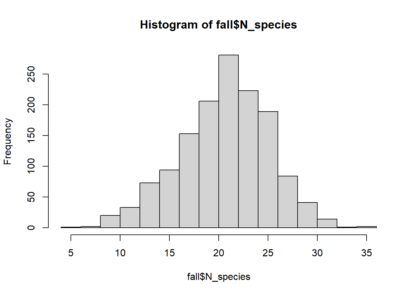
#2 choose k - let GCV find optimal
#3 autocorrelation?
# lat/long = correlated
# bottom/surface salinity = correlated
#plot(fall[,20], fall[,23])
# yes so fit w/GAMM
#4 is k large enough? diagnostics ok?
# diagnostic/residual plots; QQ,resid vs. pred
# take care when interpretting results
# k-index; further below 1 = missed pattern in resids
# k is too low if edf ~ k'
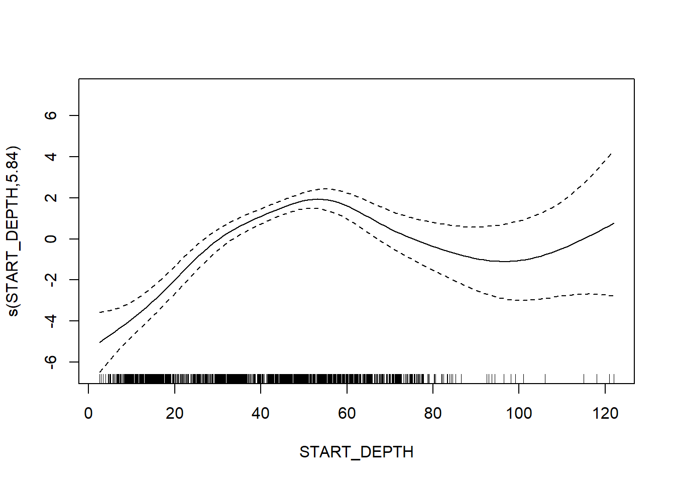
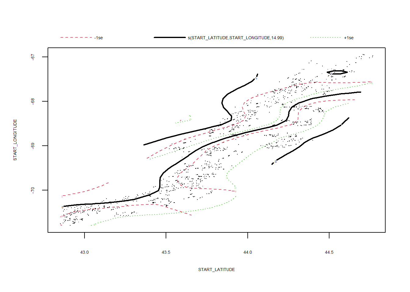
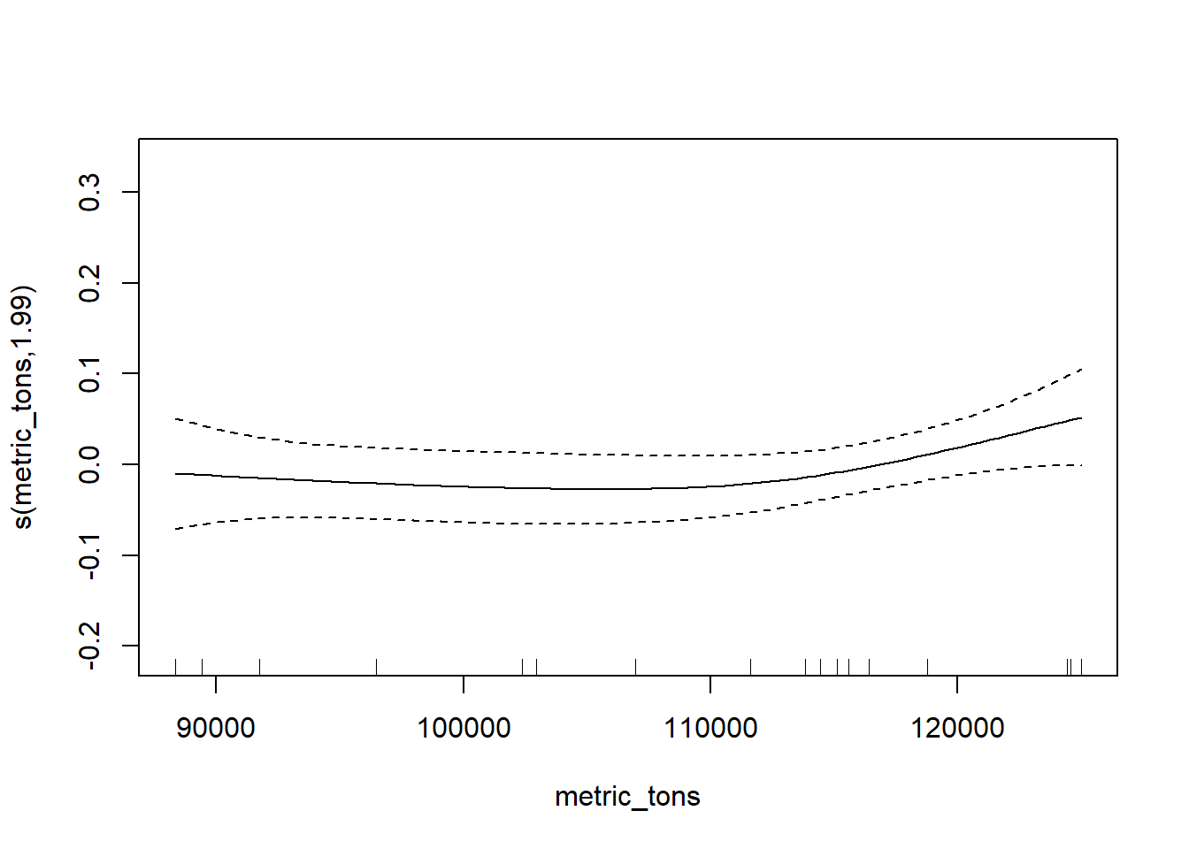
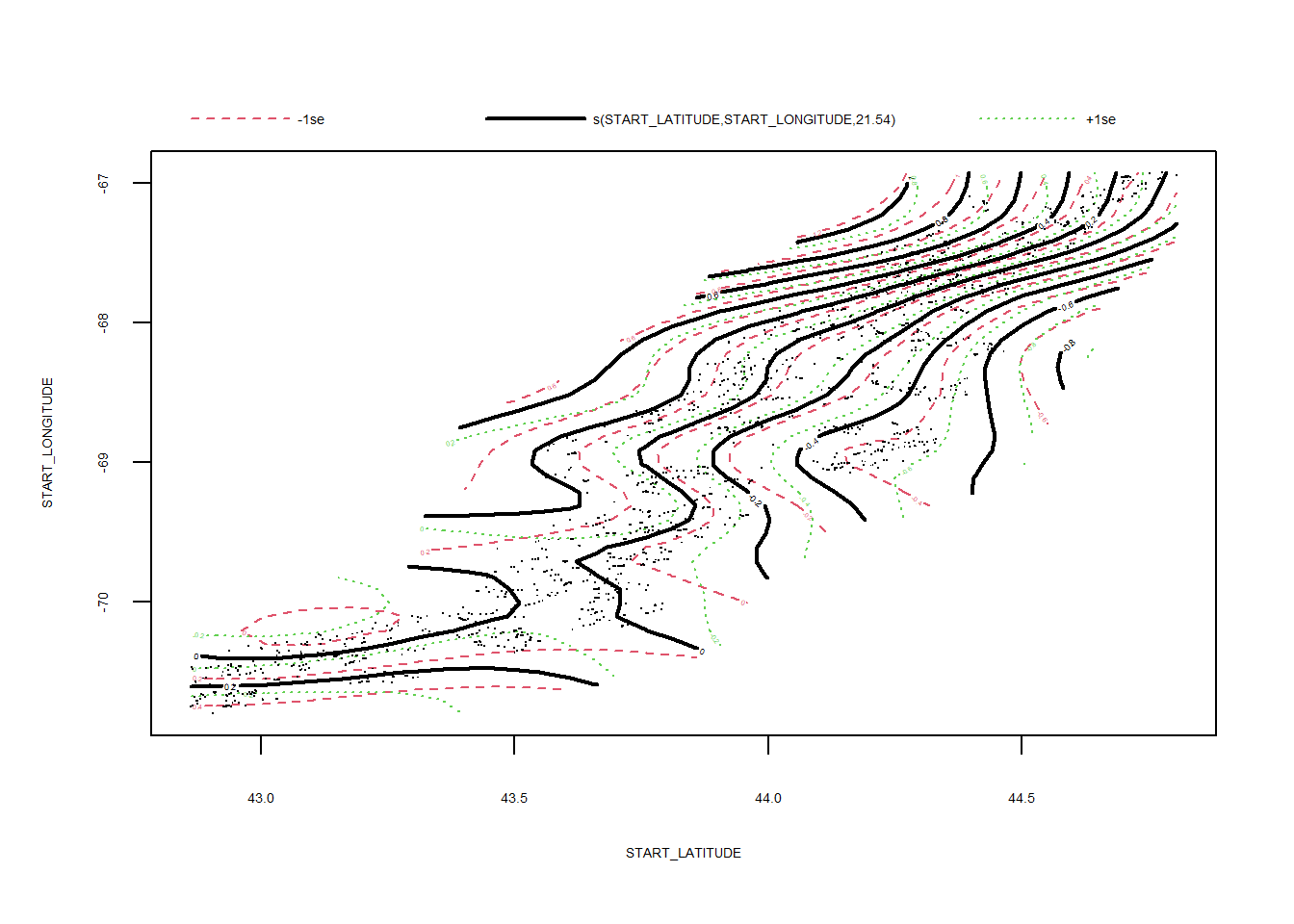
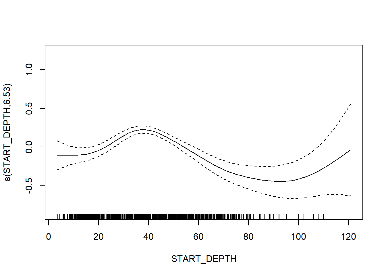
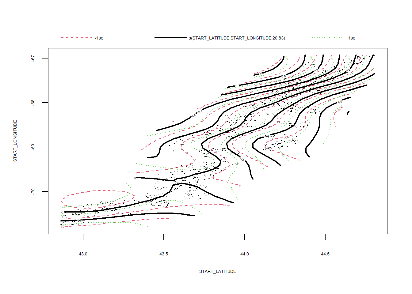
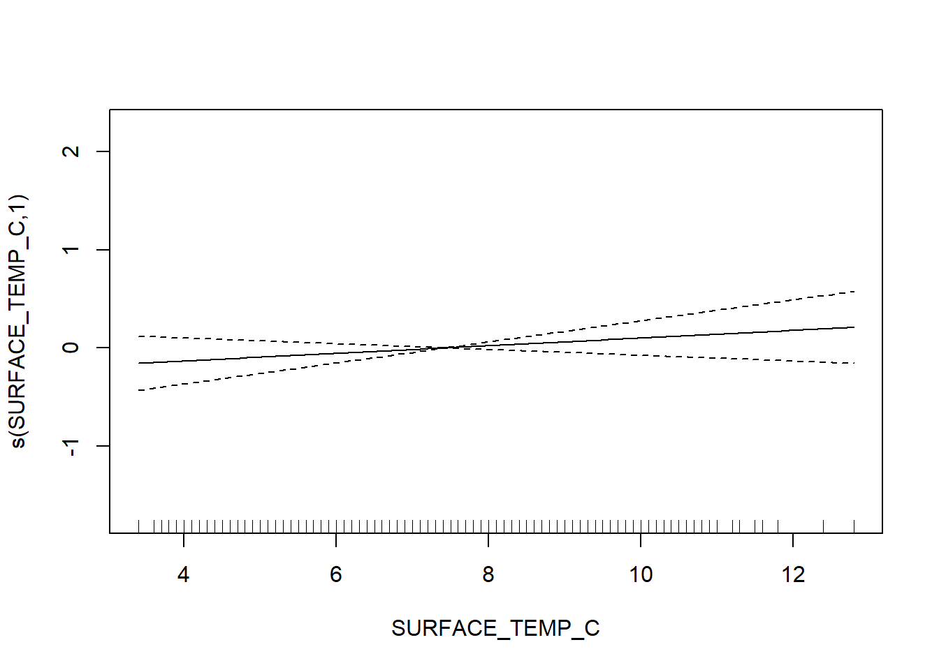
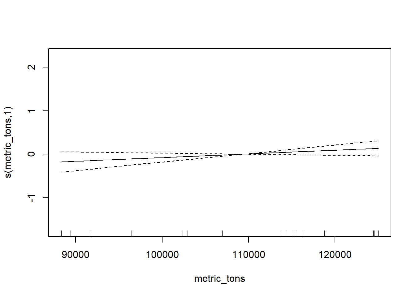
## best model fit is N_Fall_2
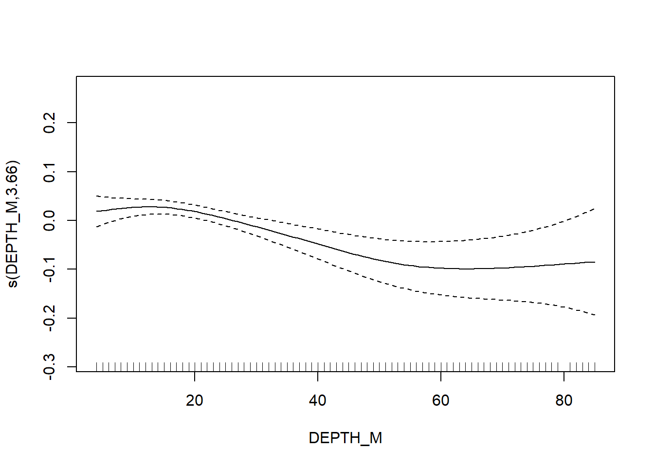
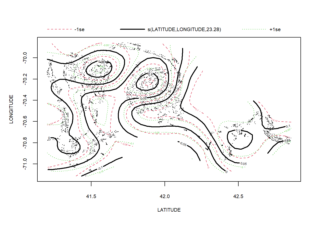
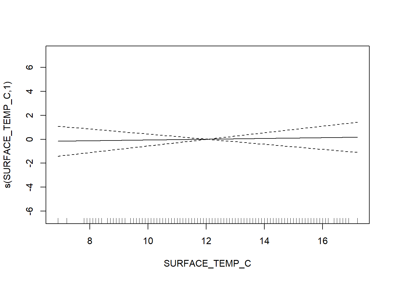
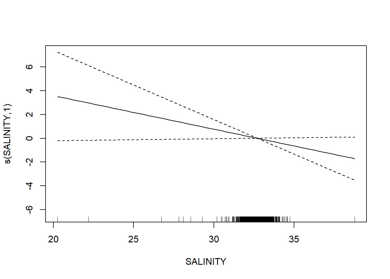
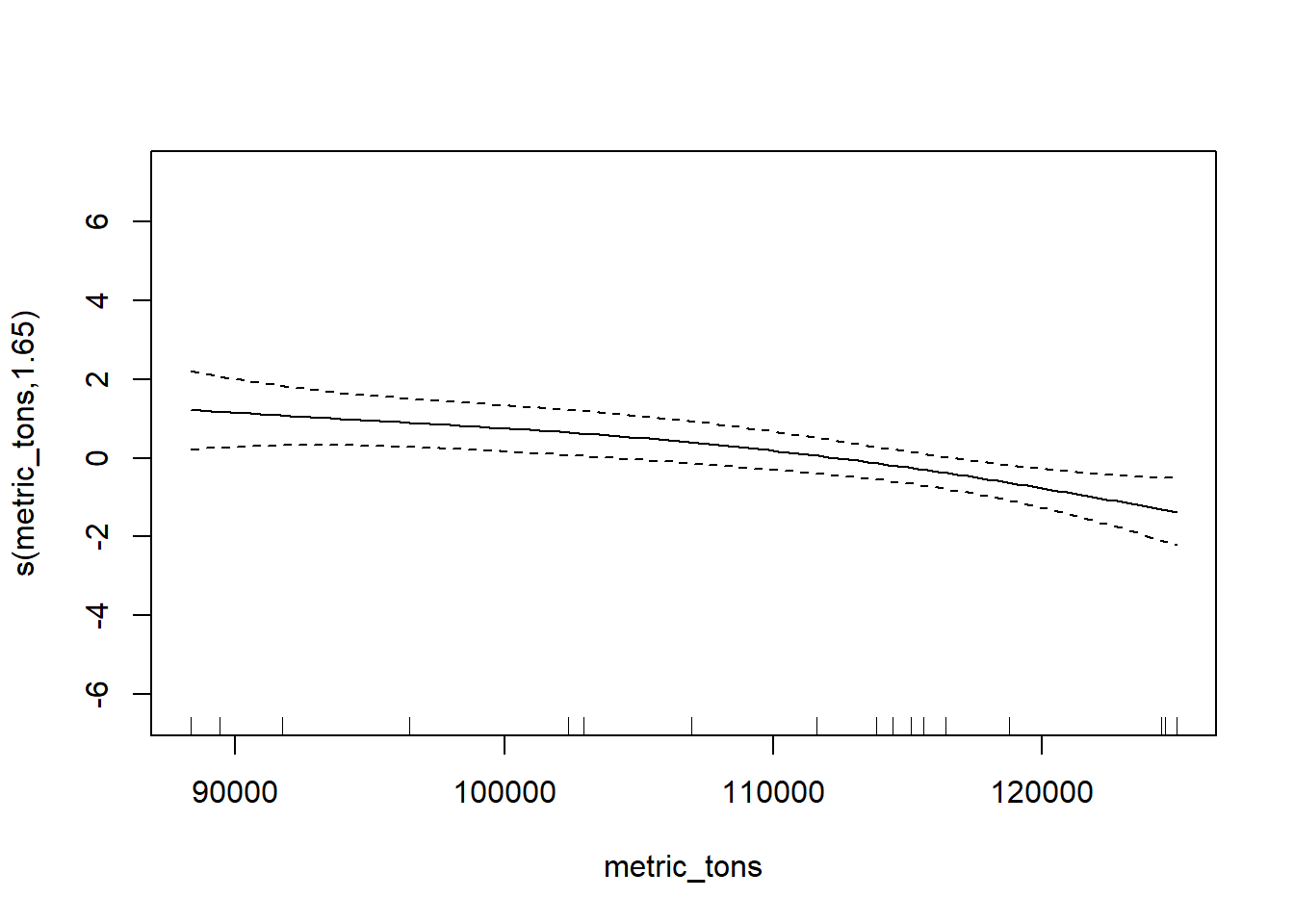
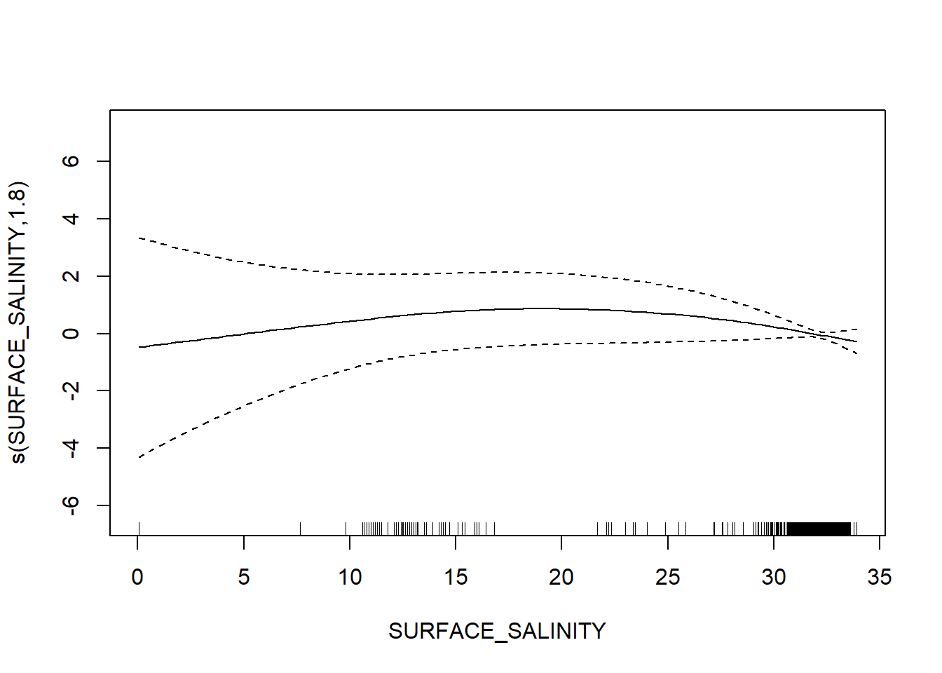
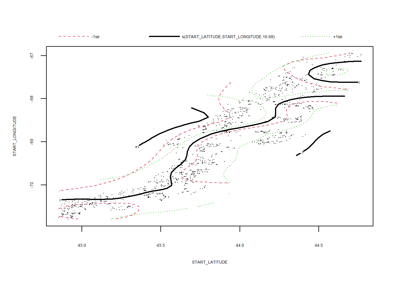
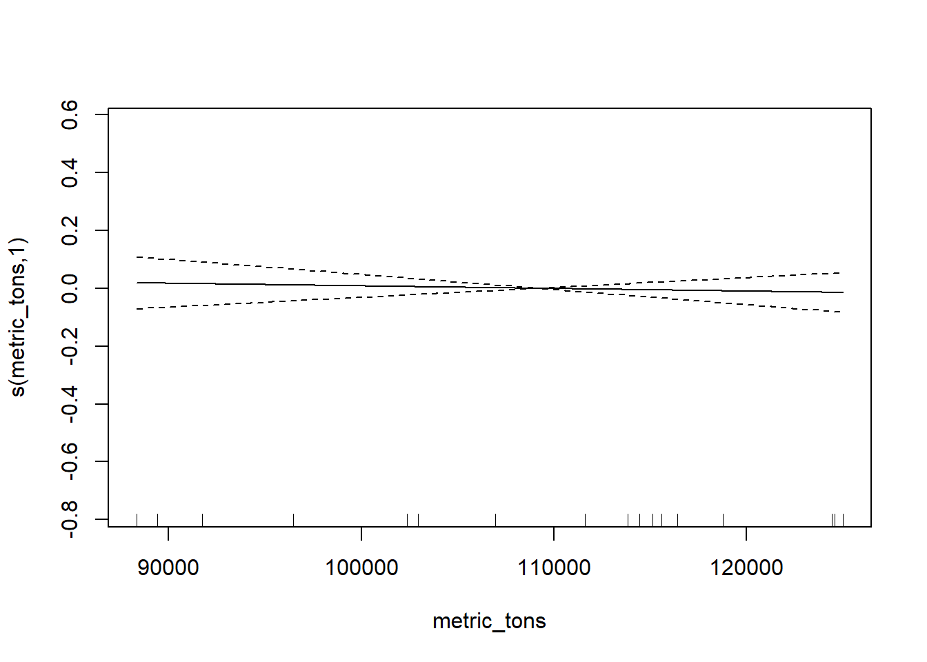
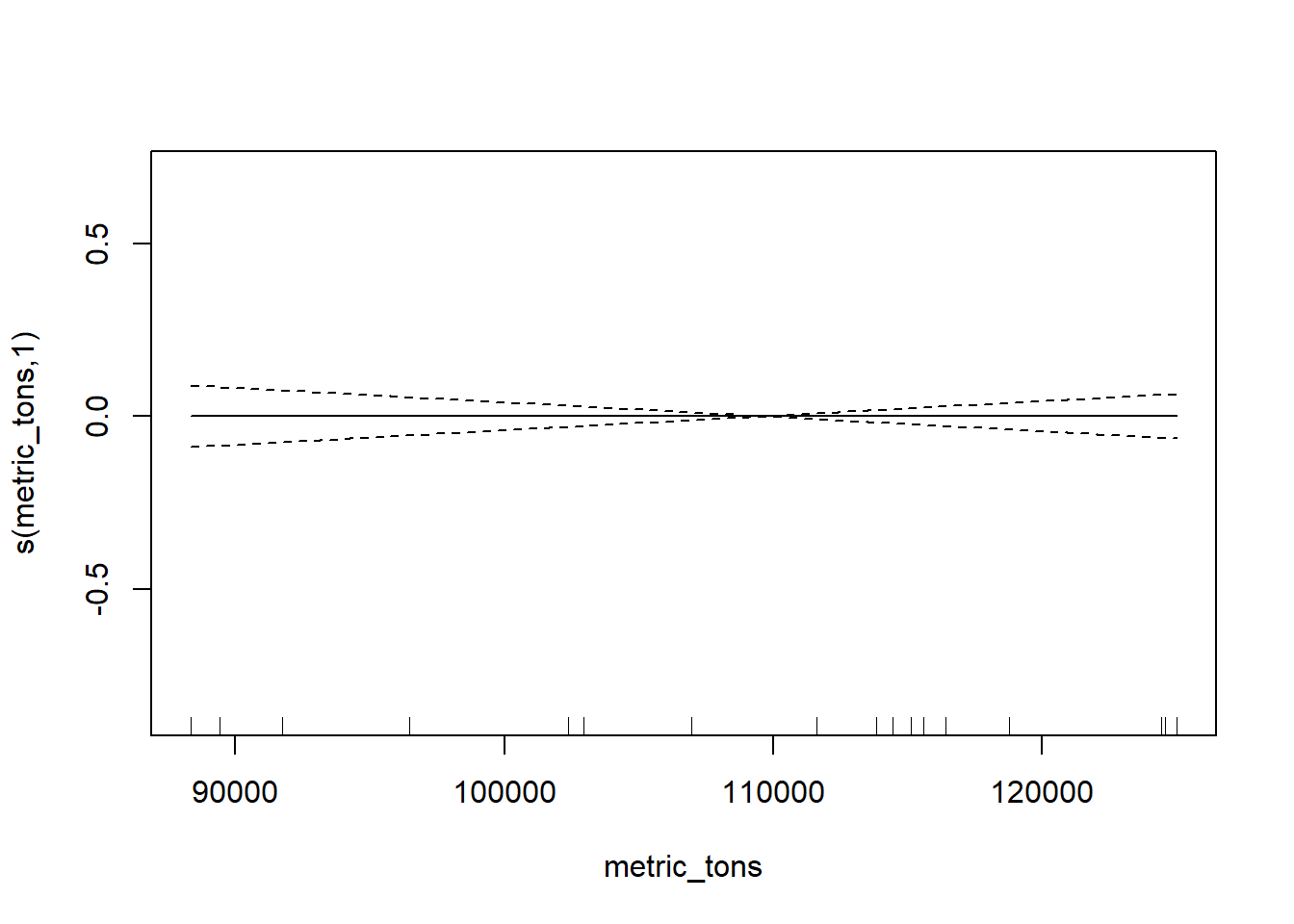
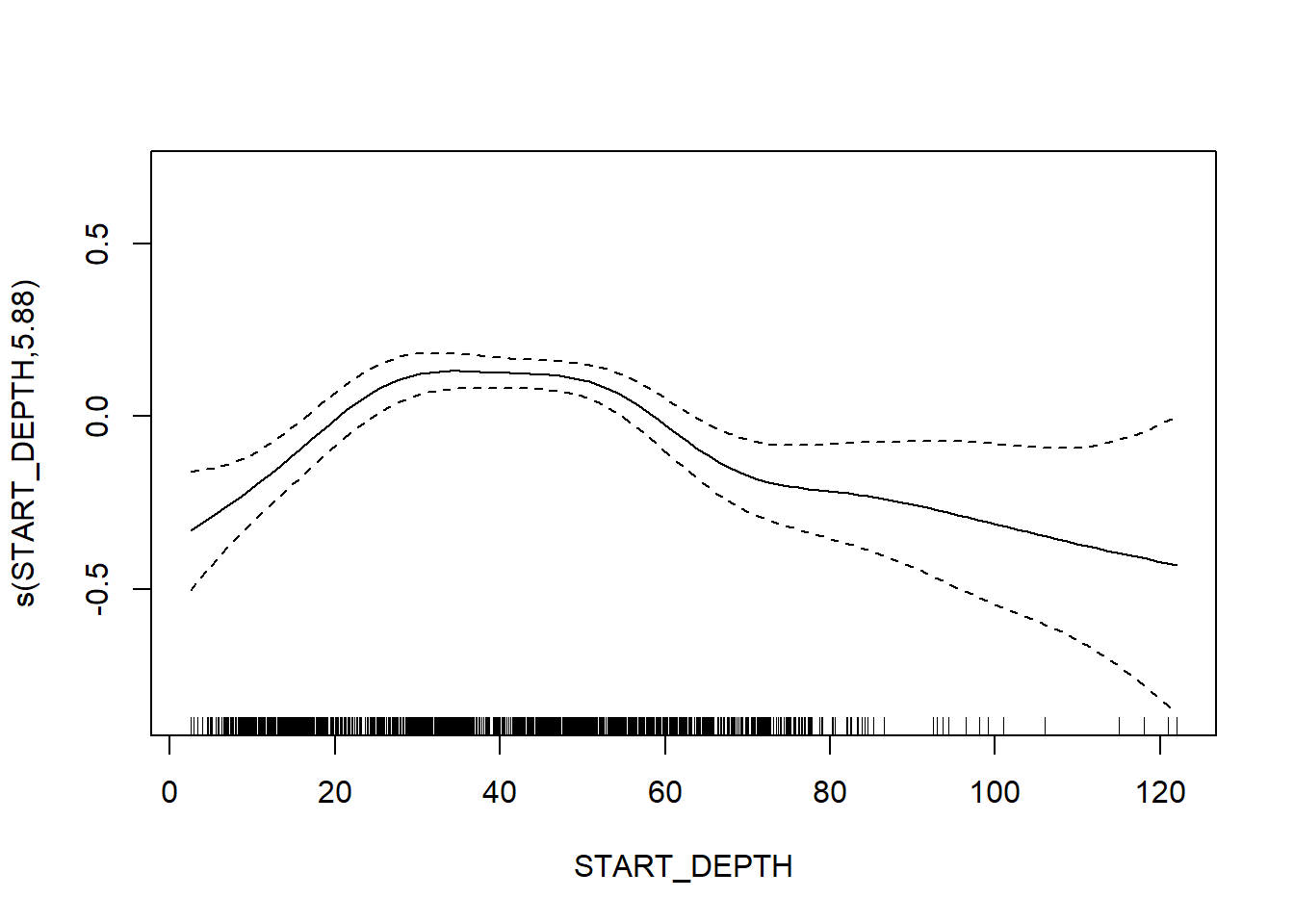
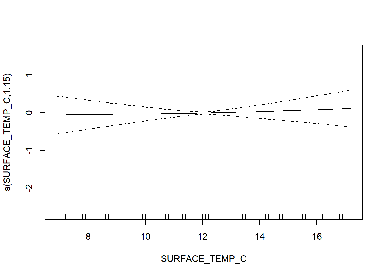
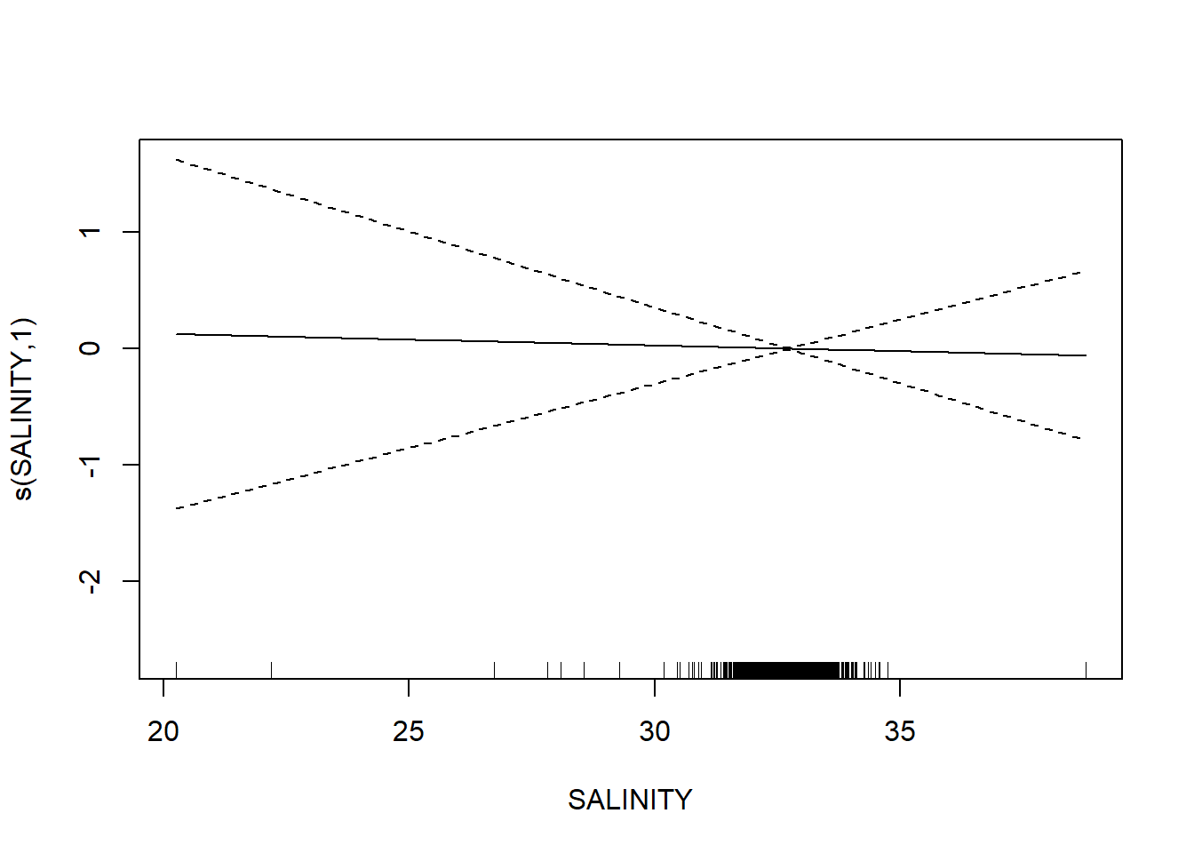
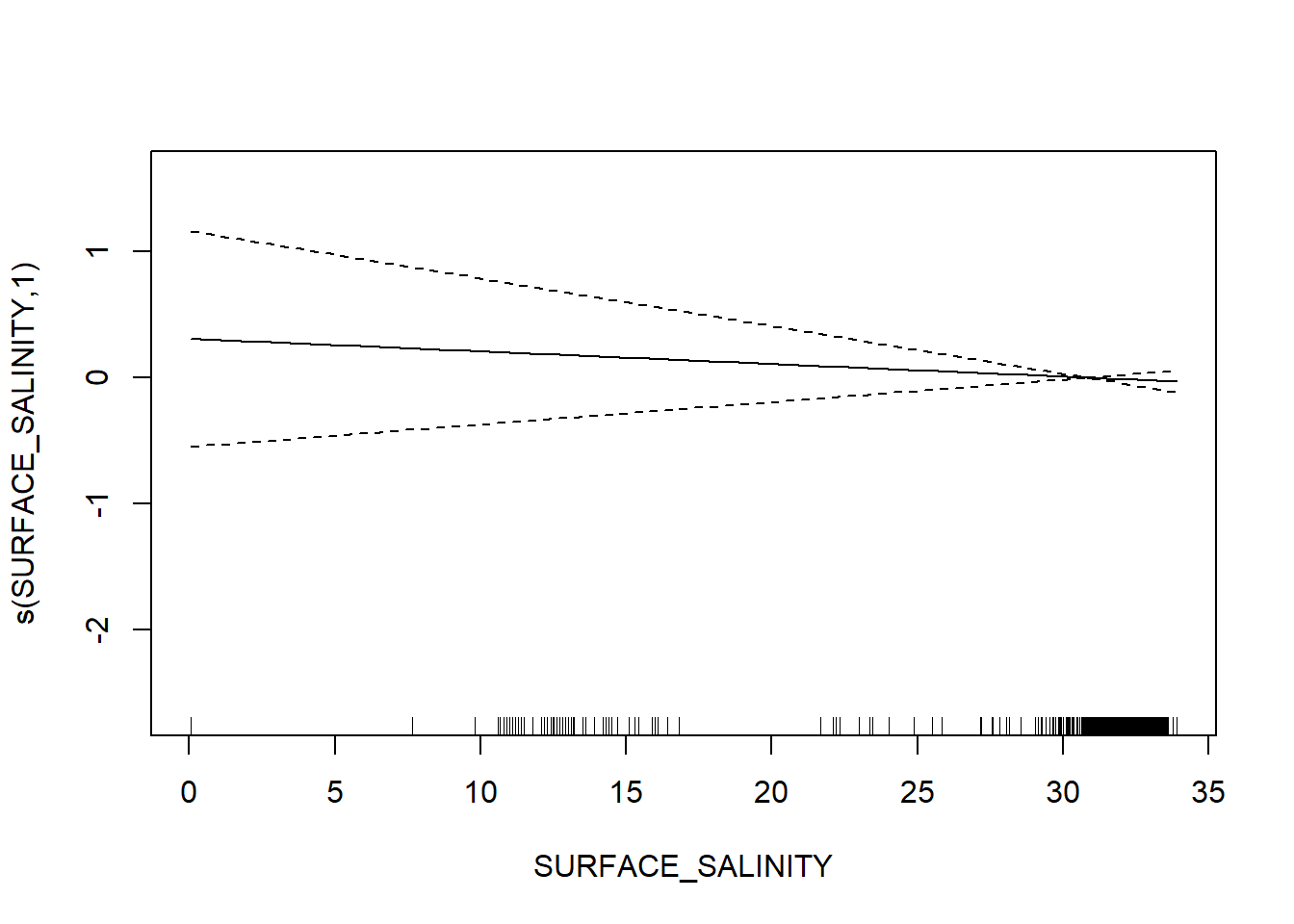
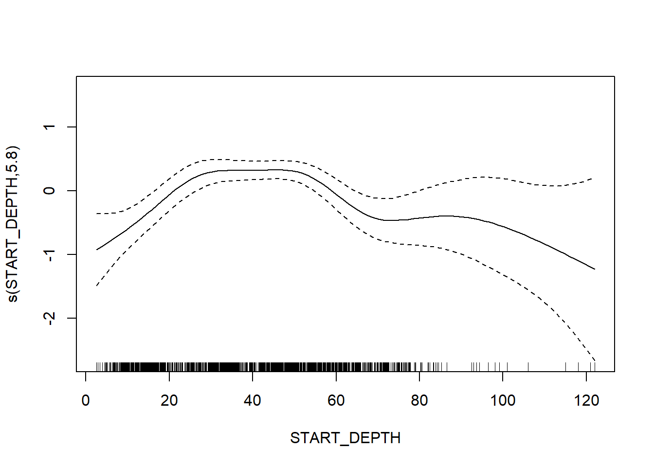
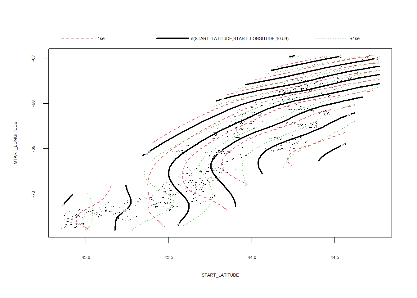
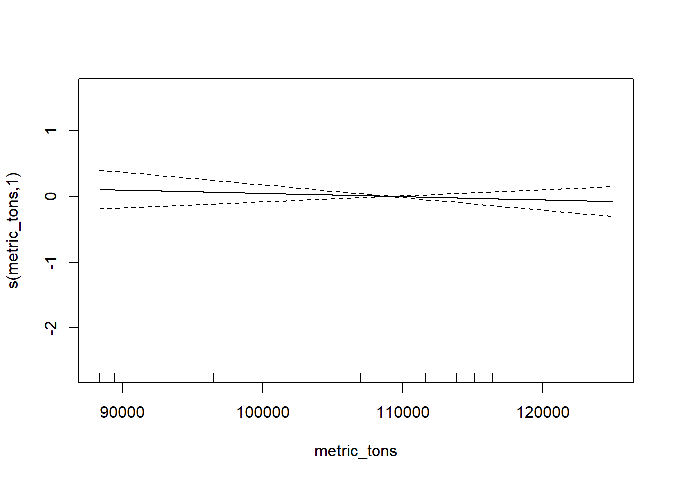
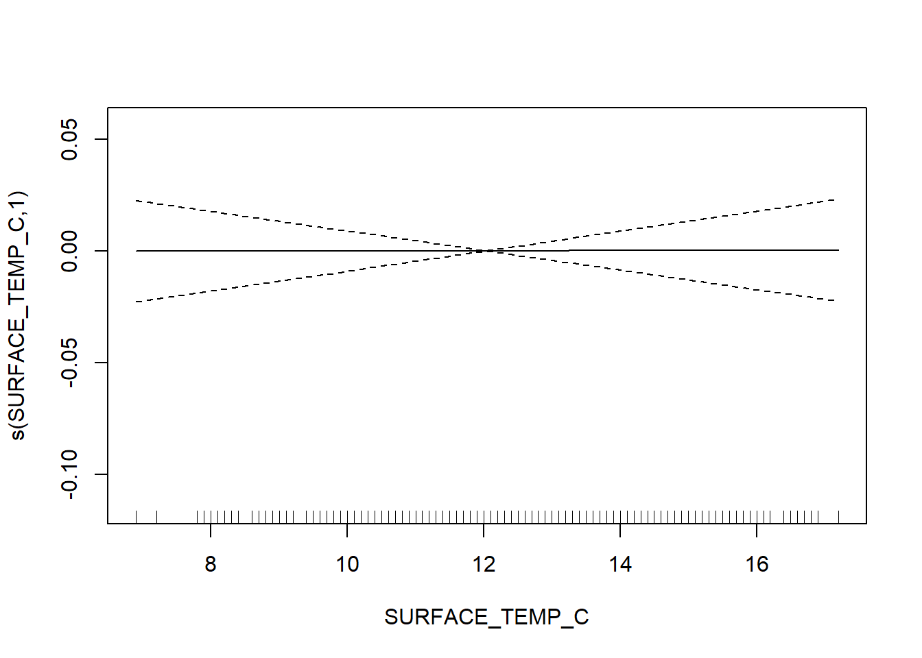
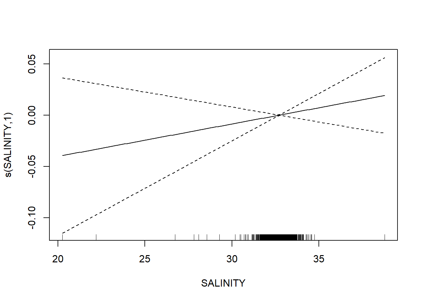
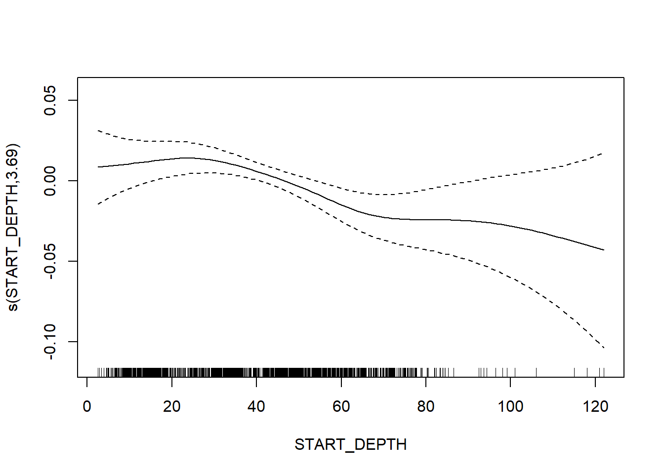
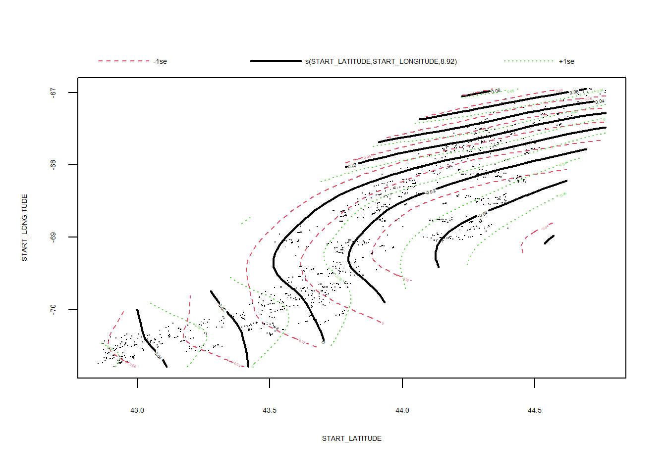
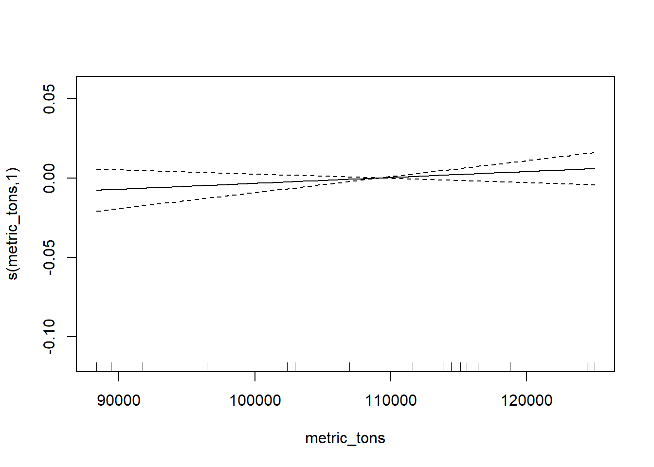
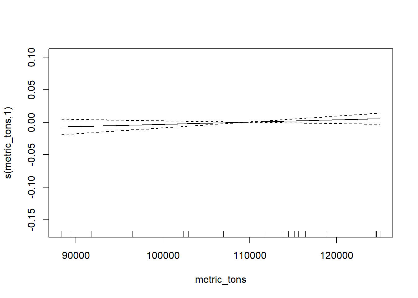
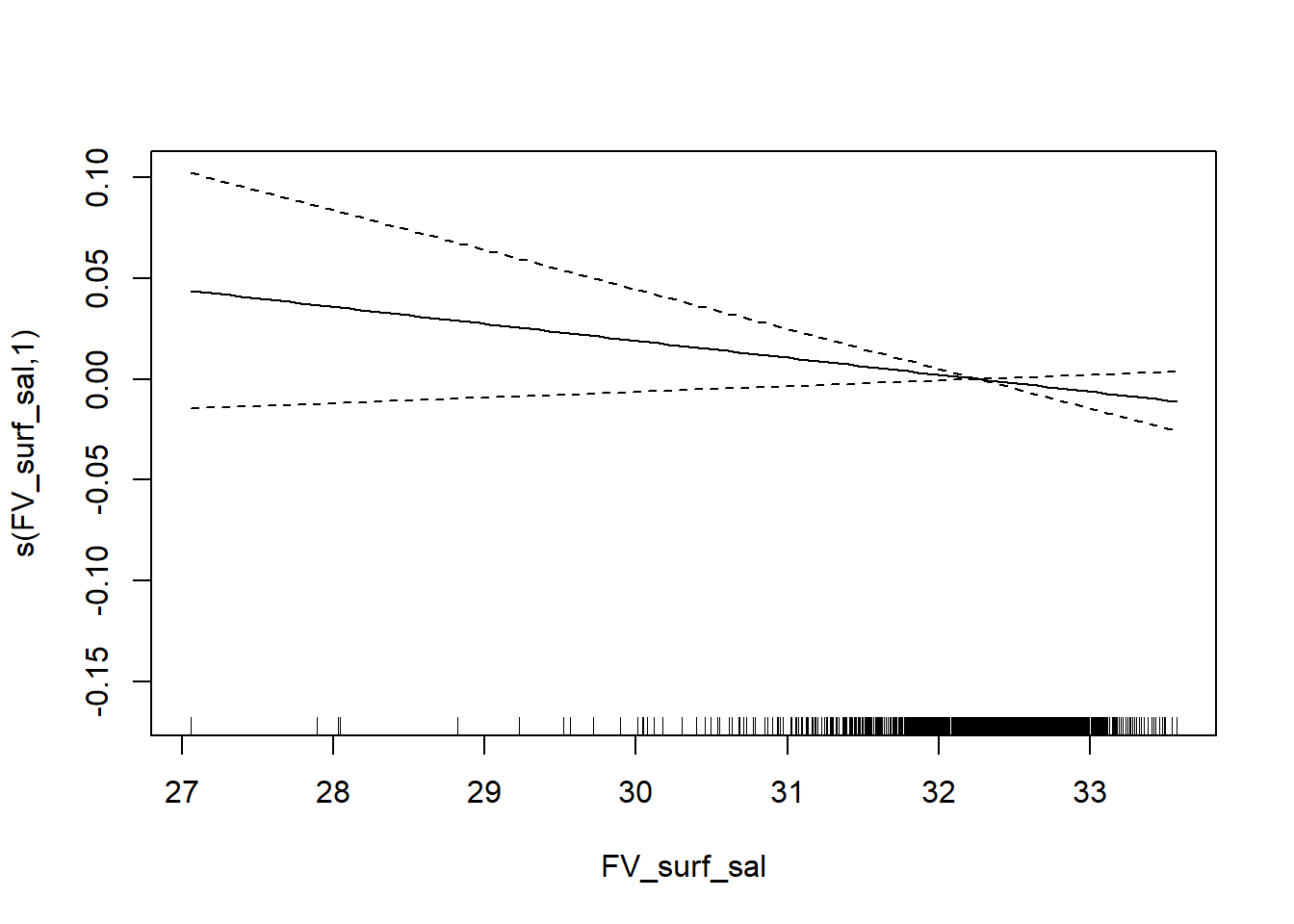
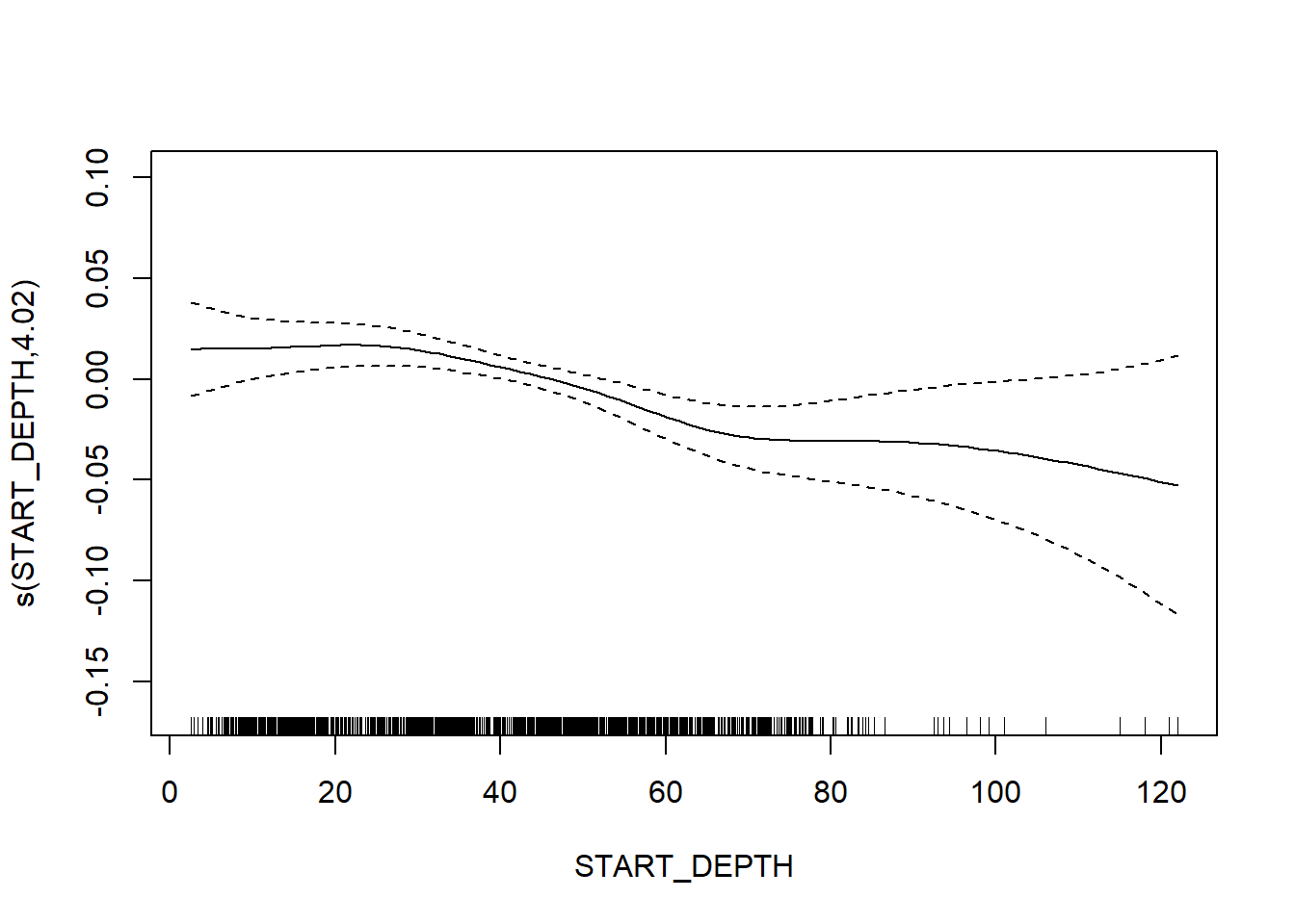
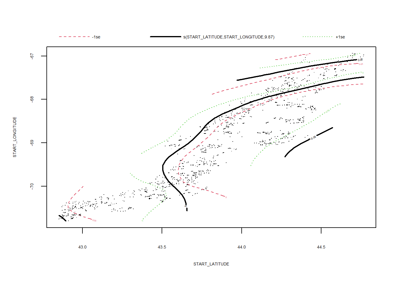
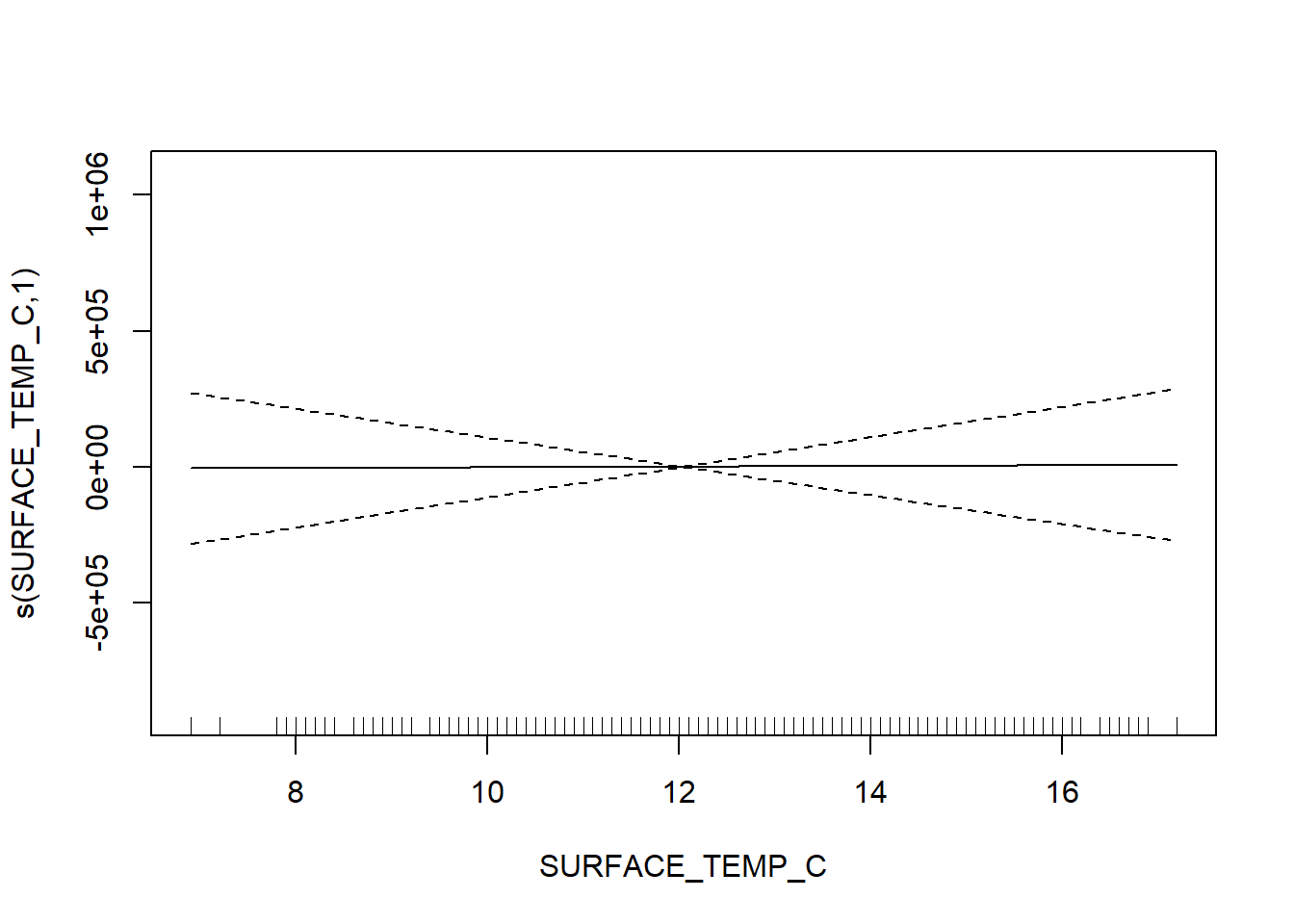
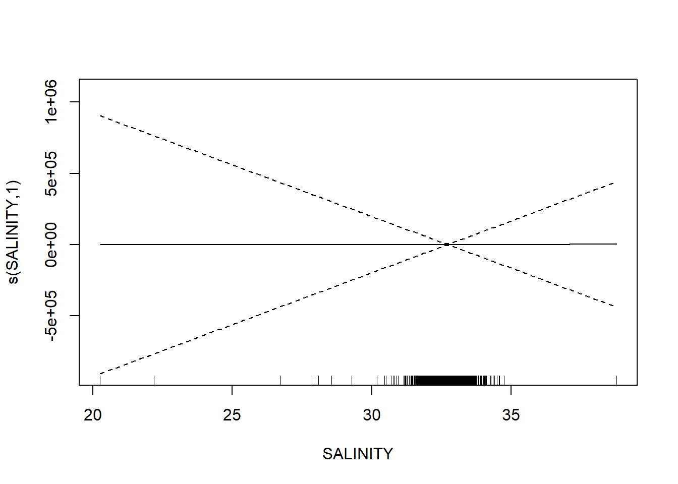
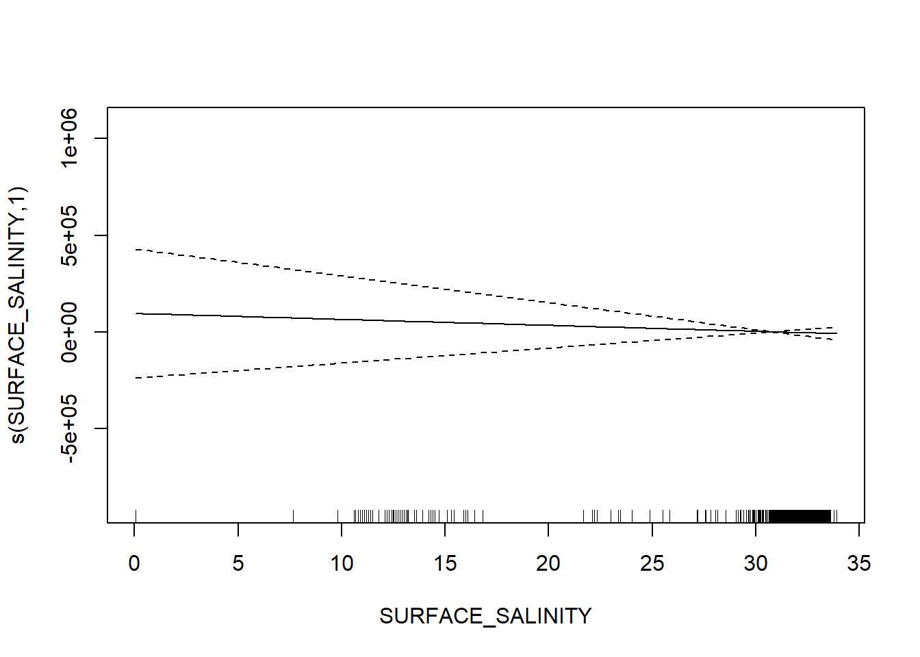
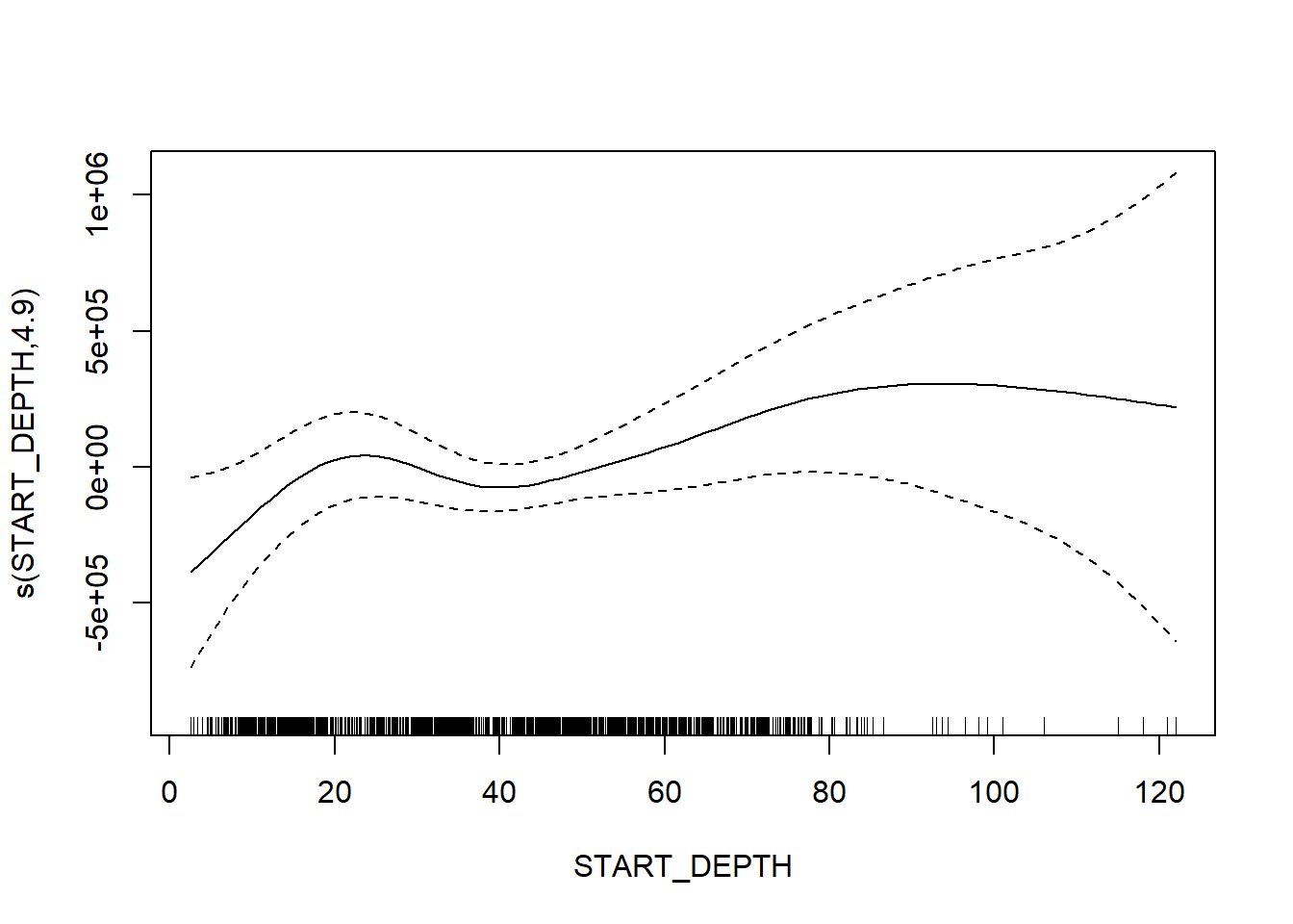
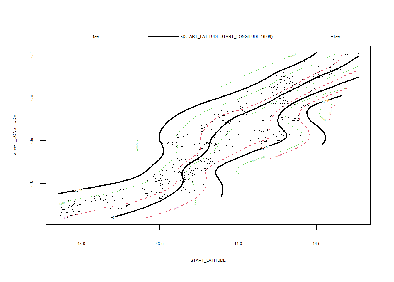
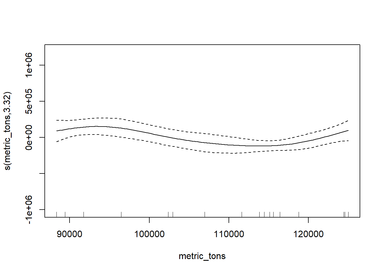
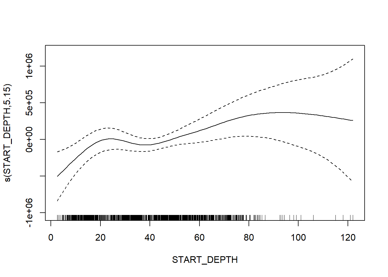
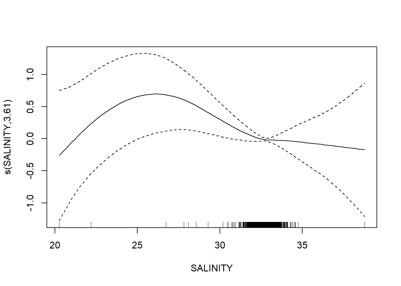
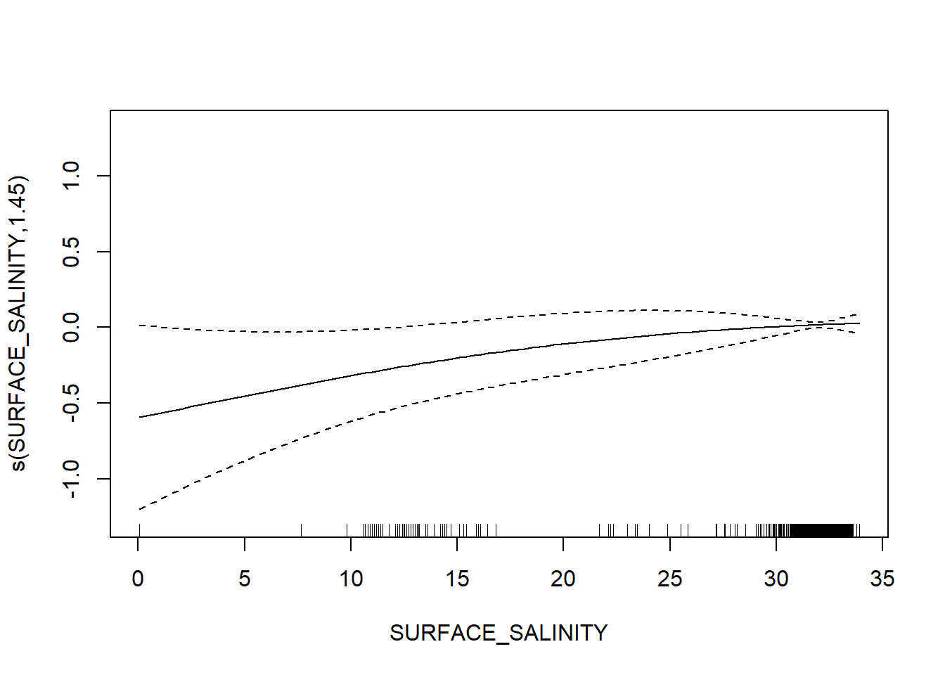
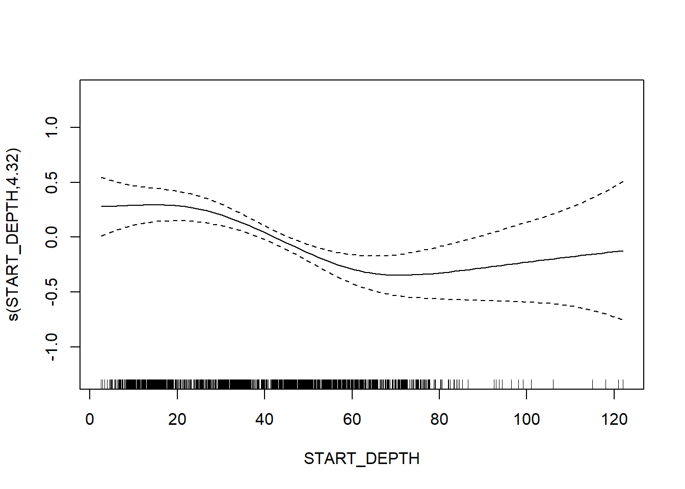
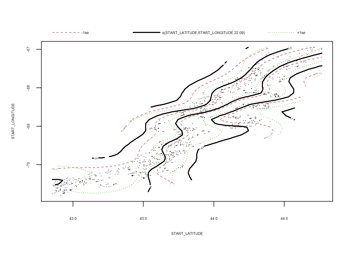
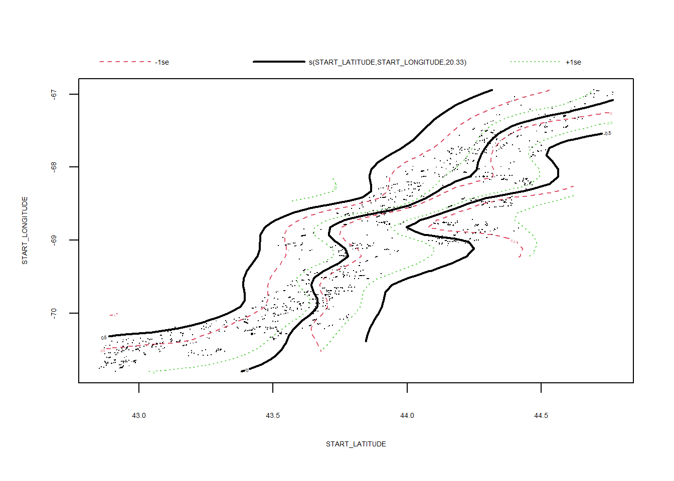
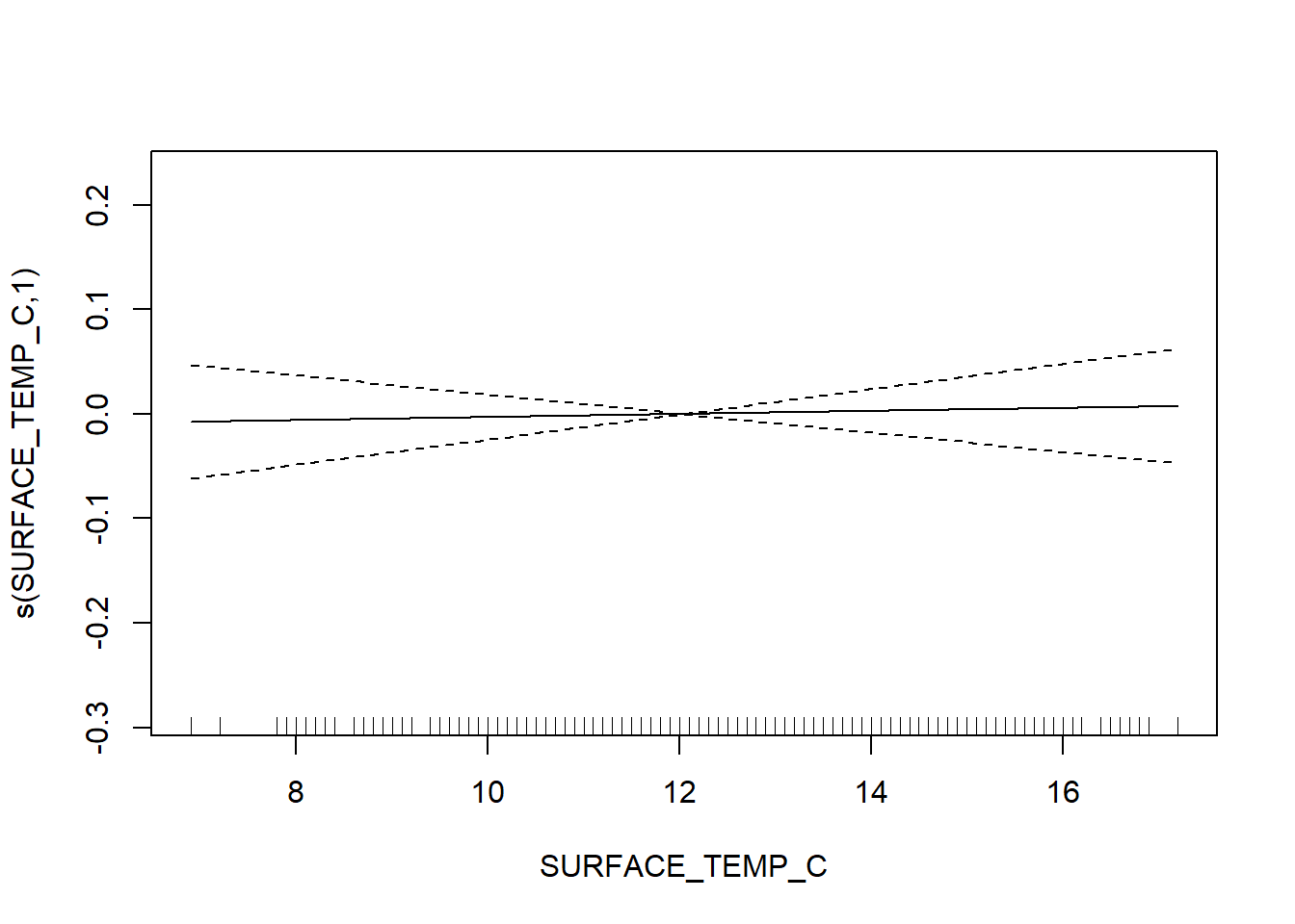
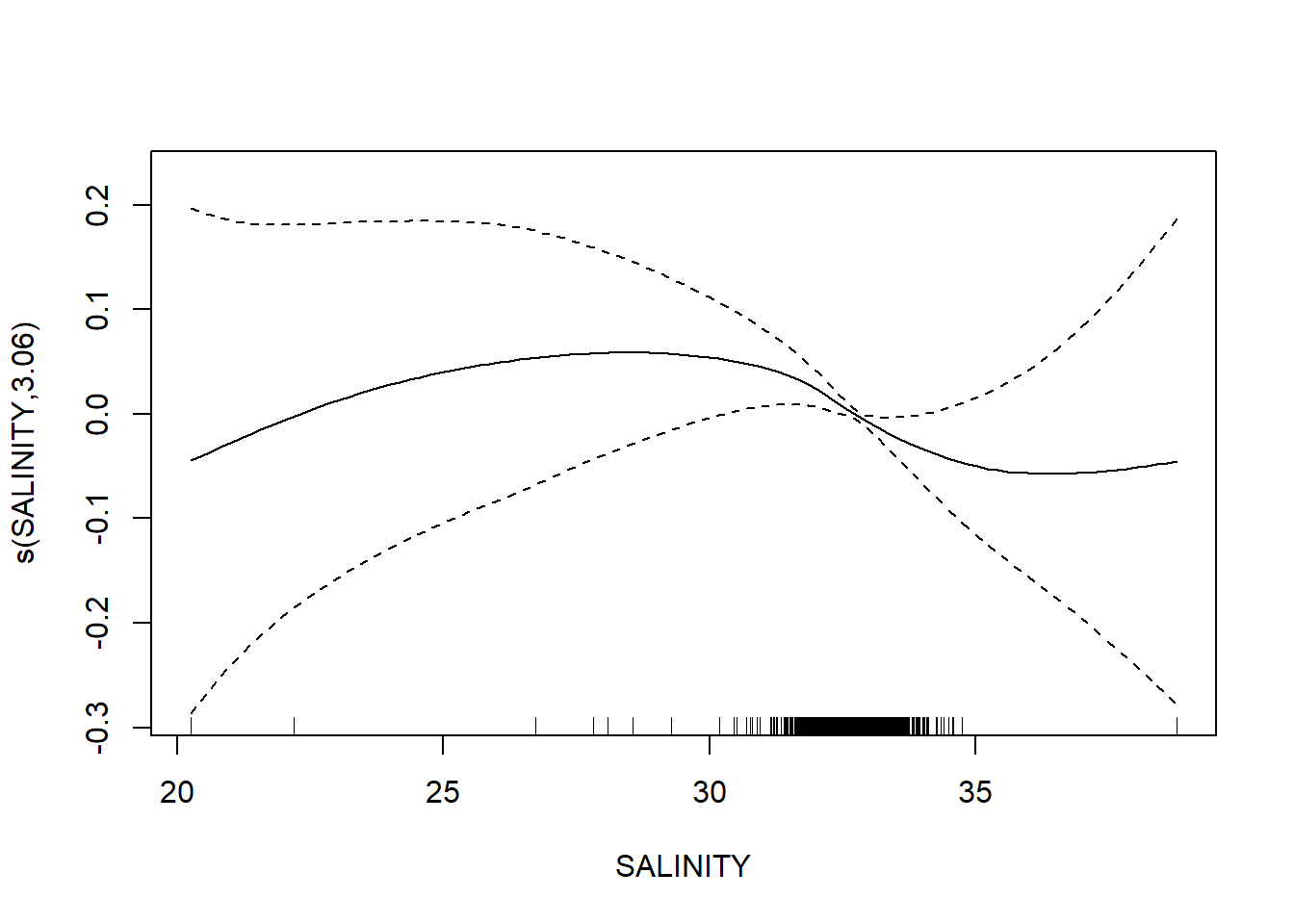
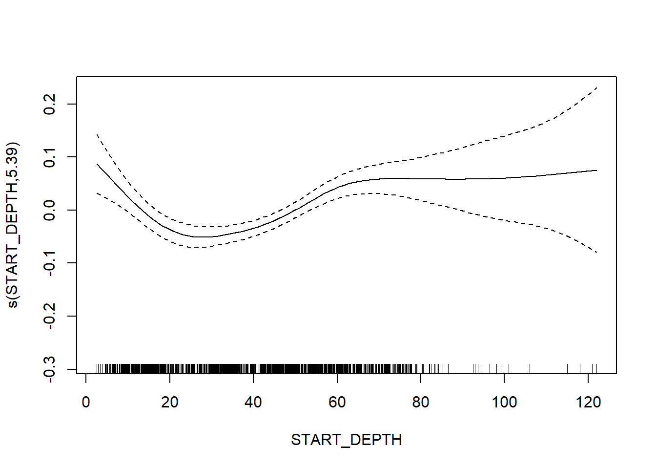
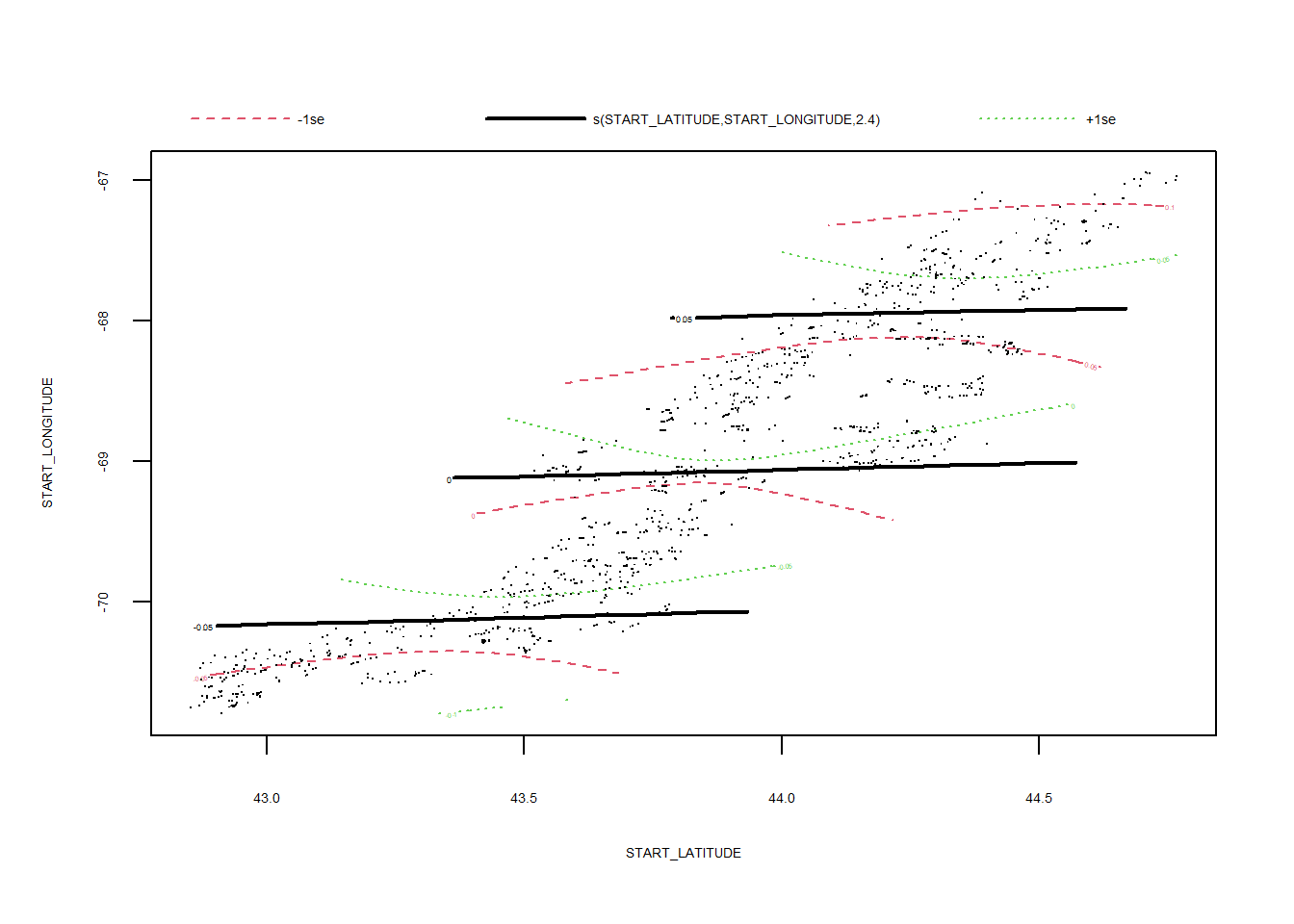
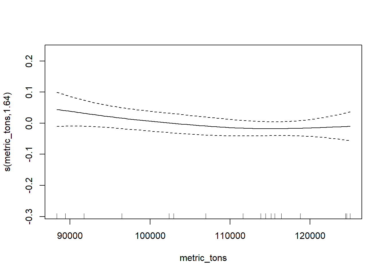
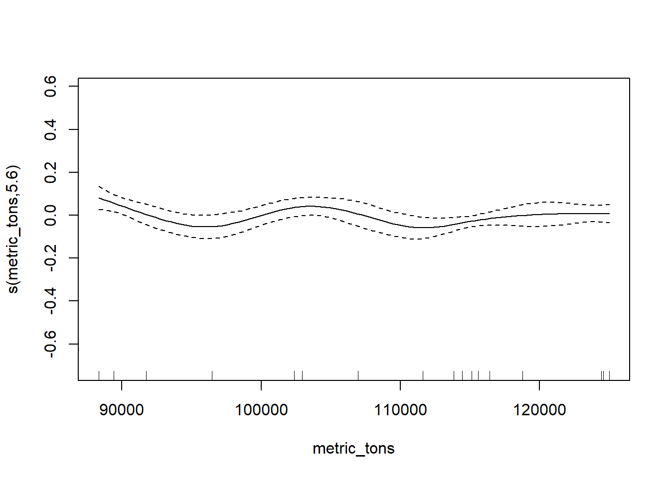
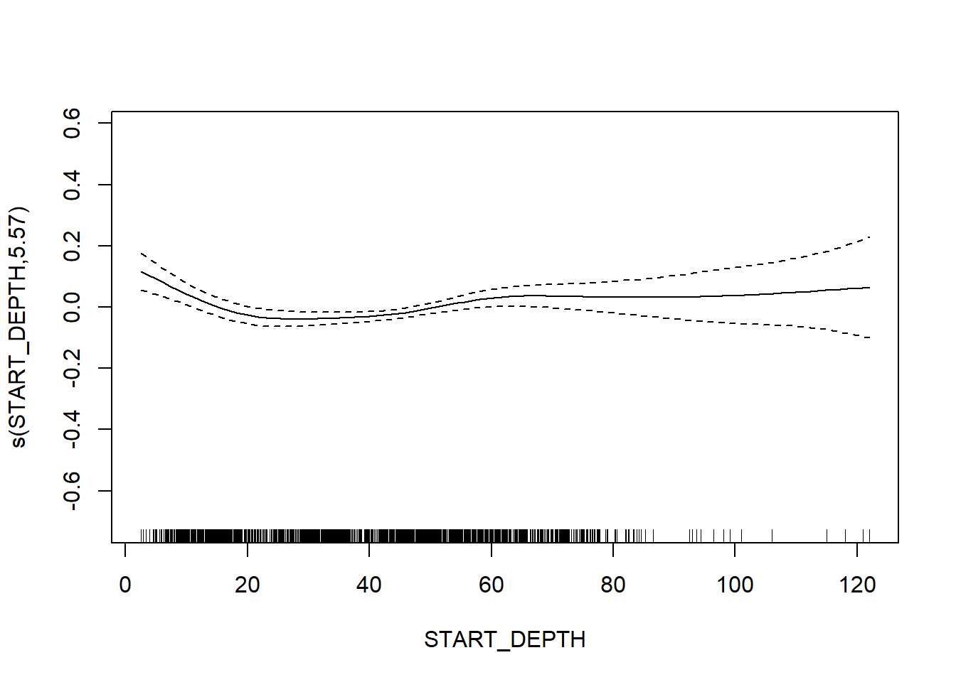
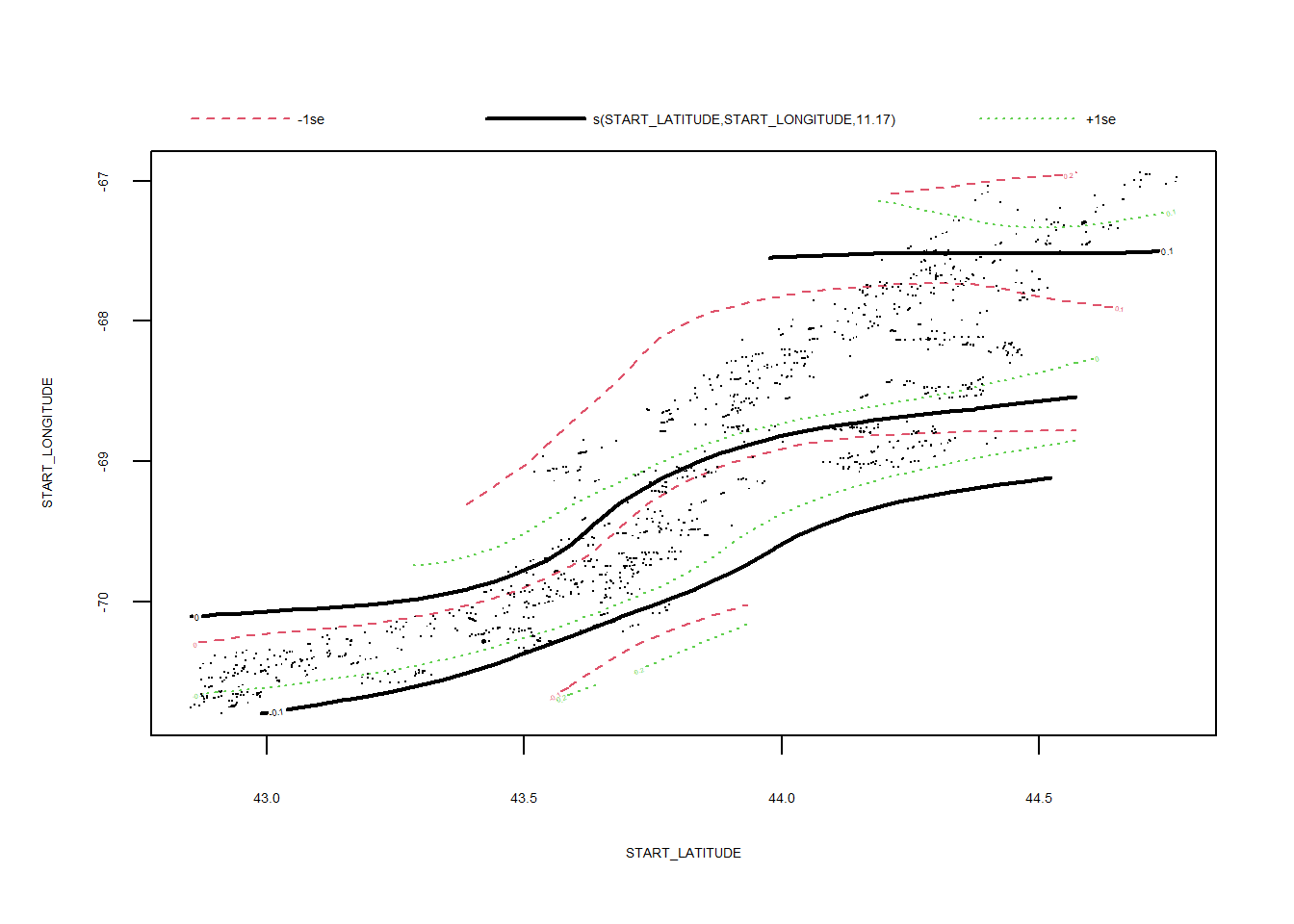
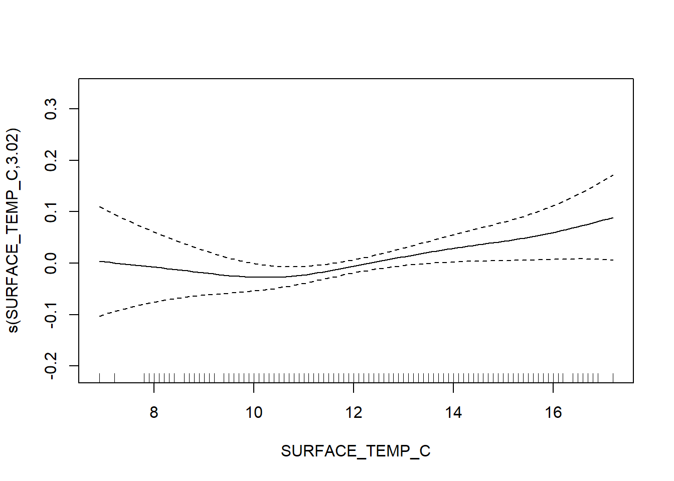
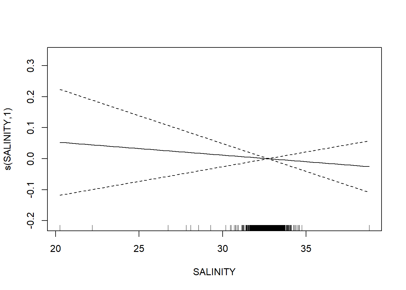
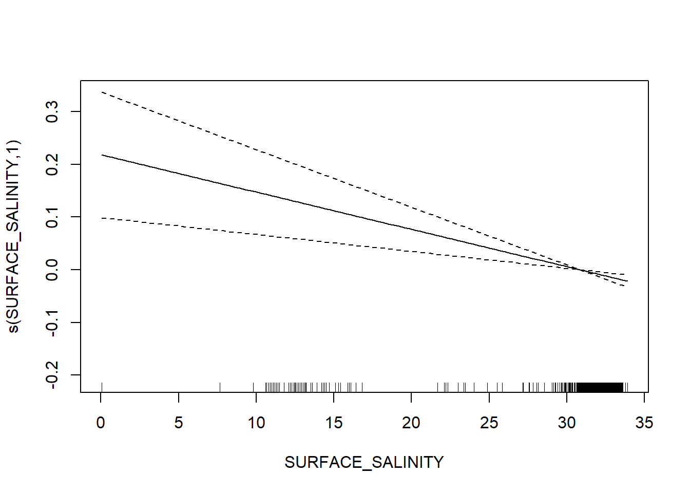
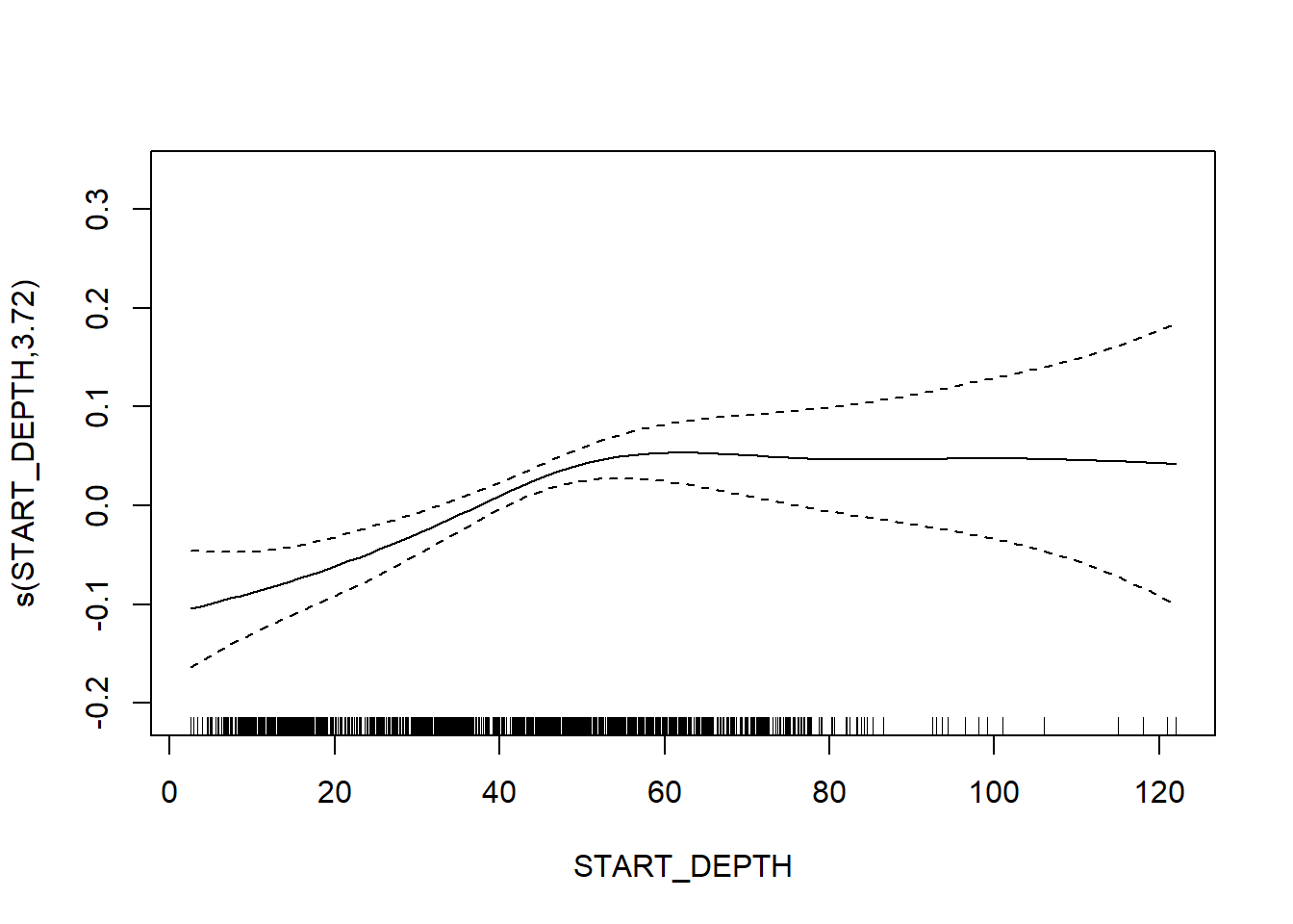
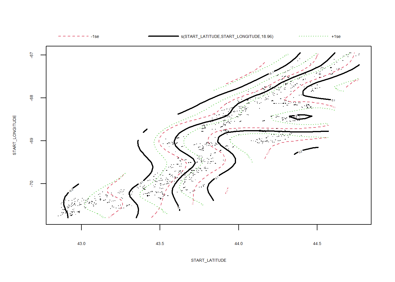
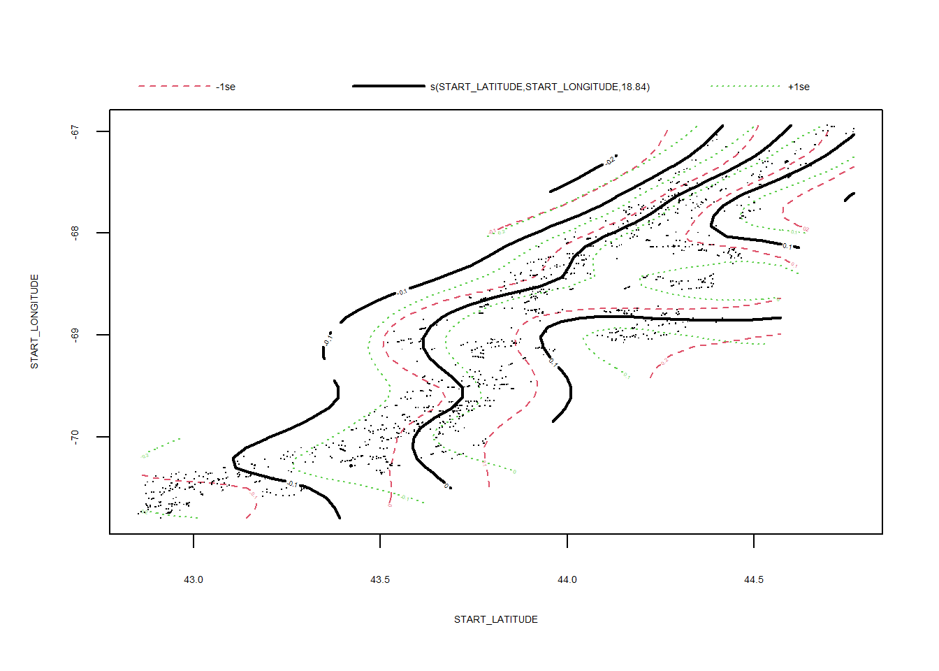
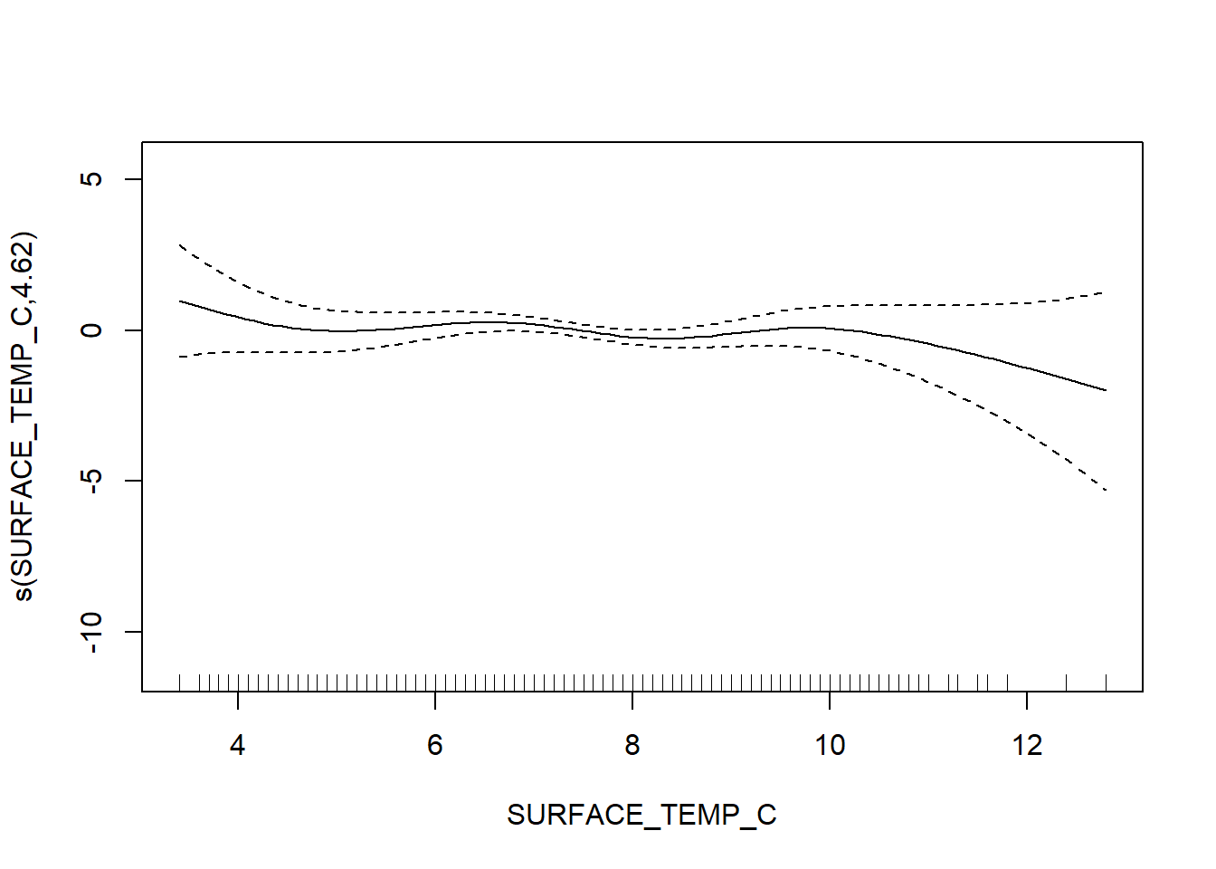
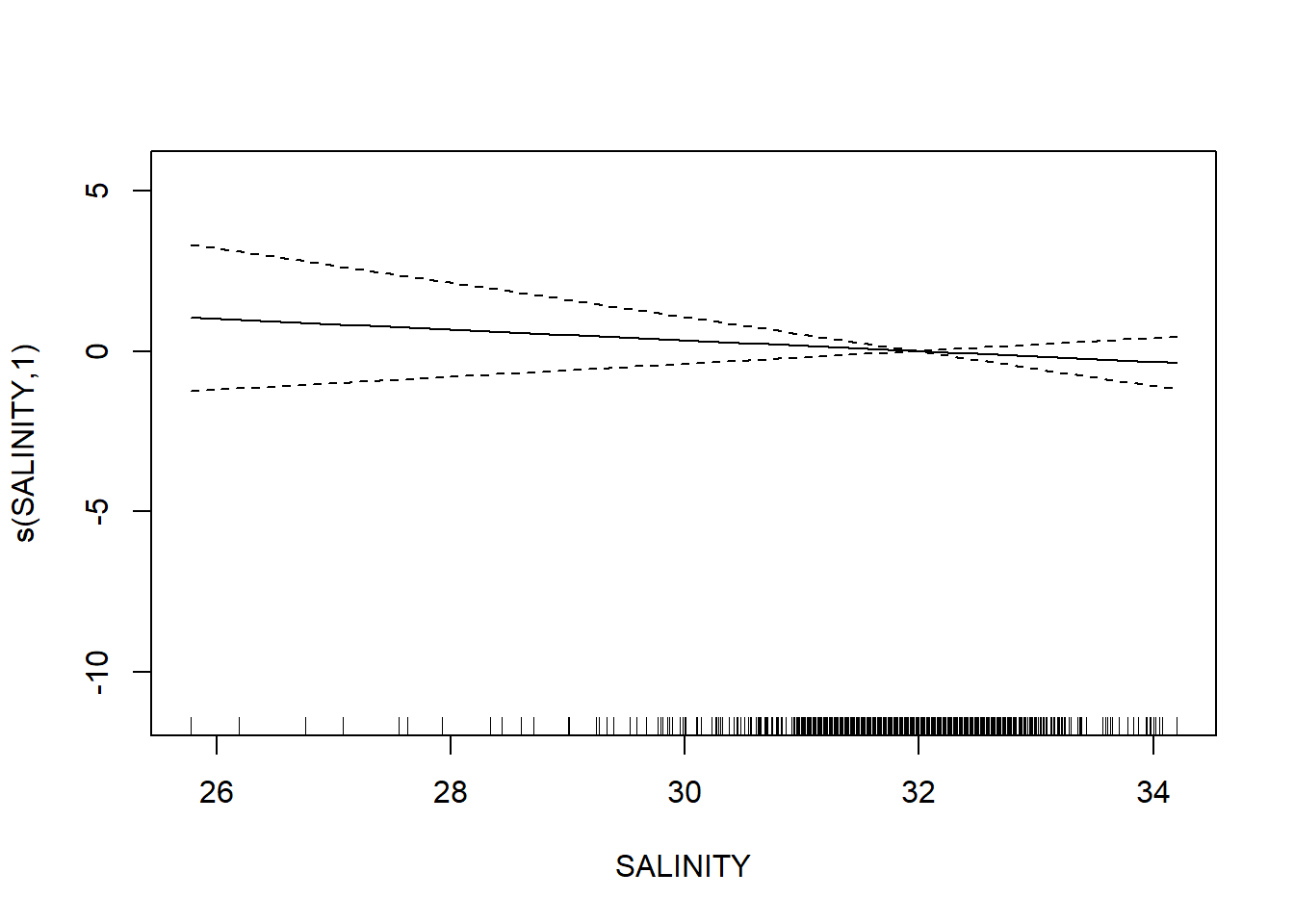
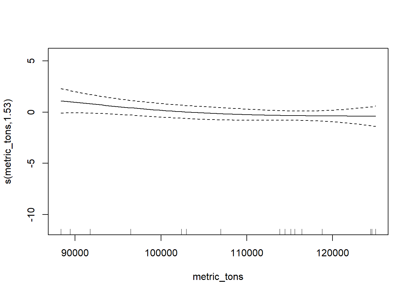
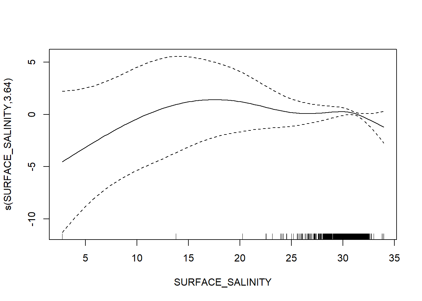
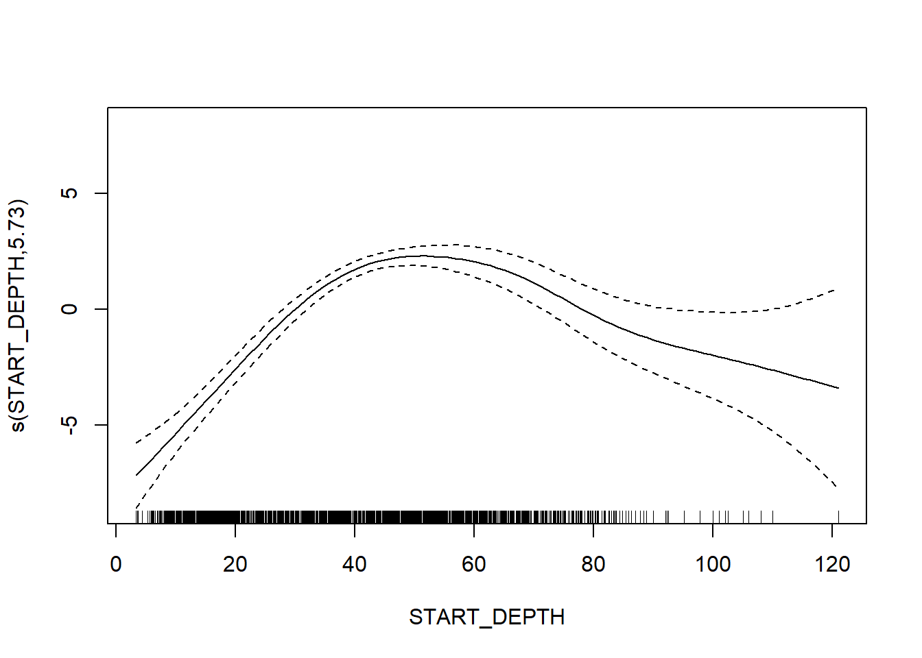
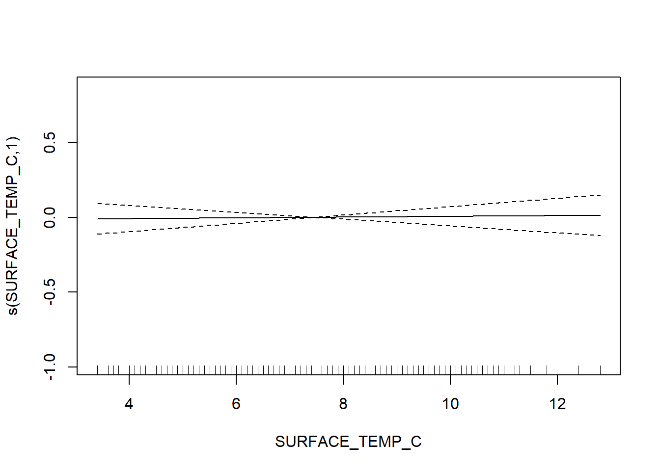
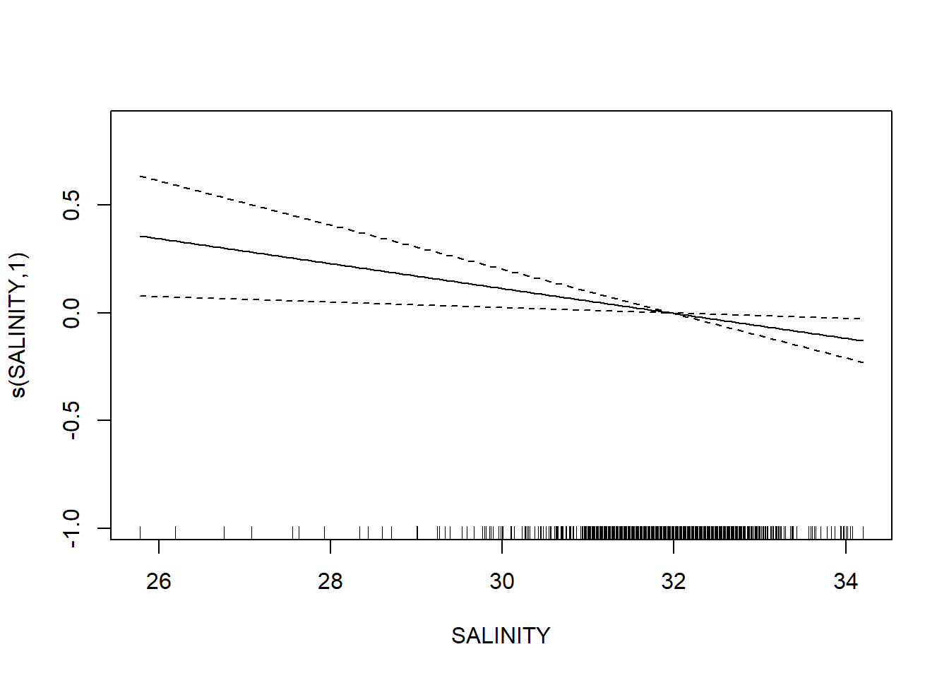
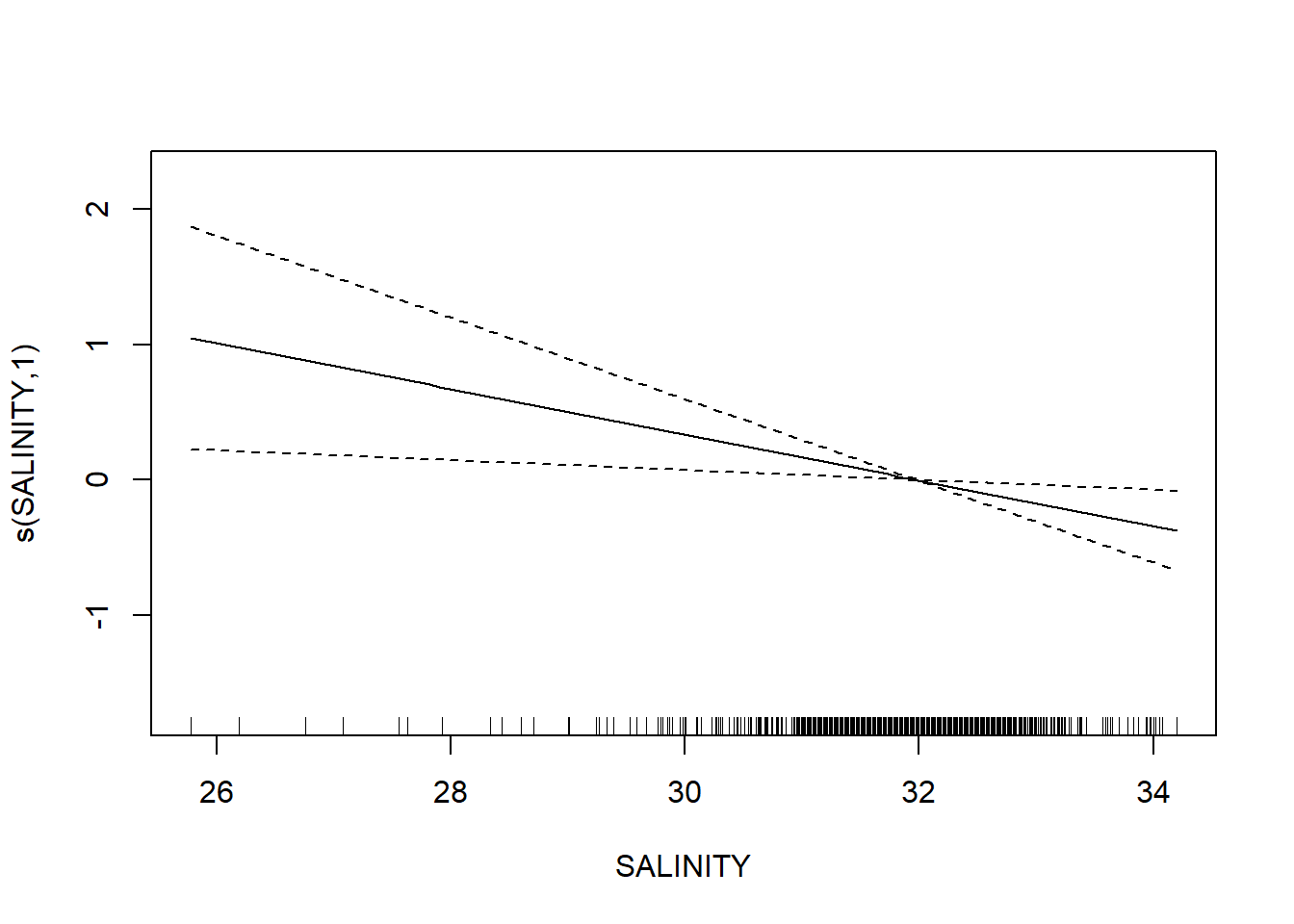
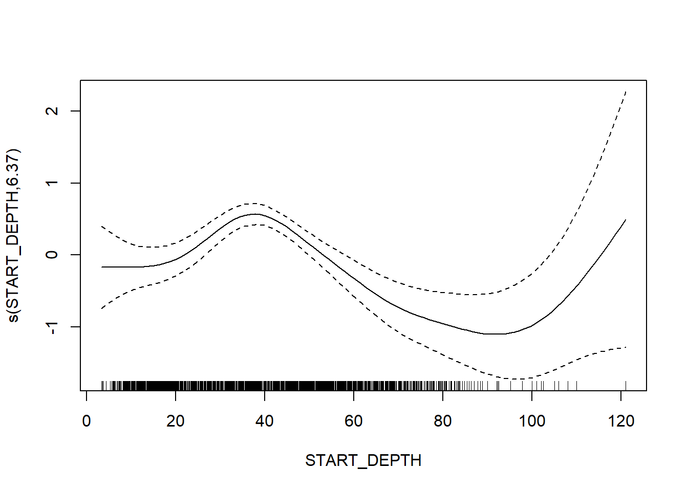
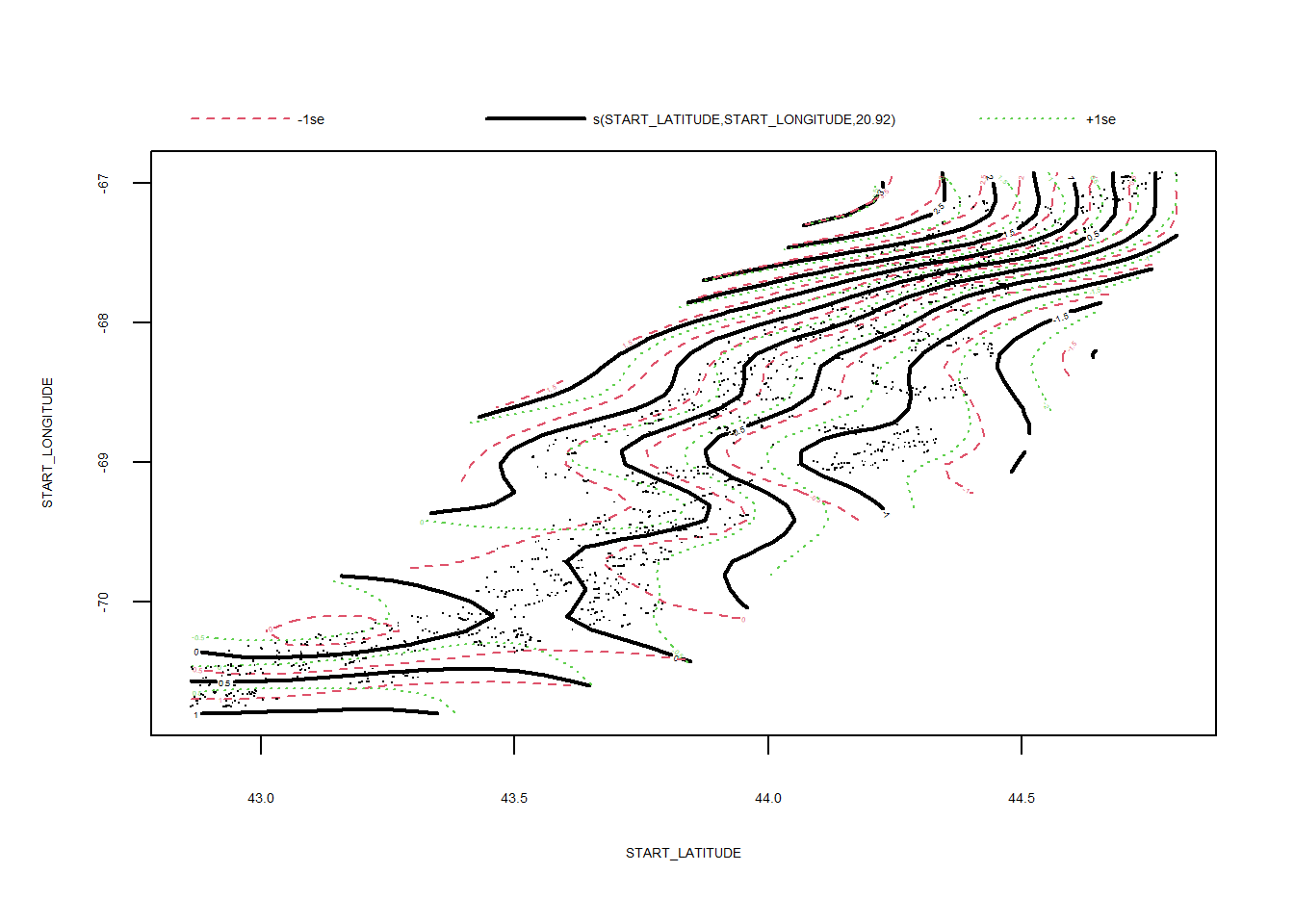
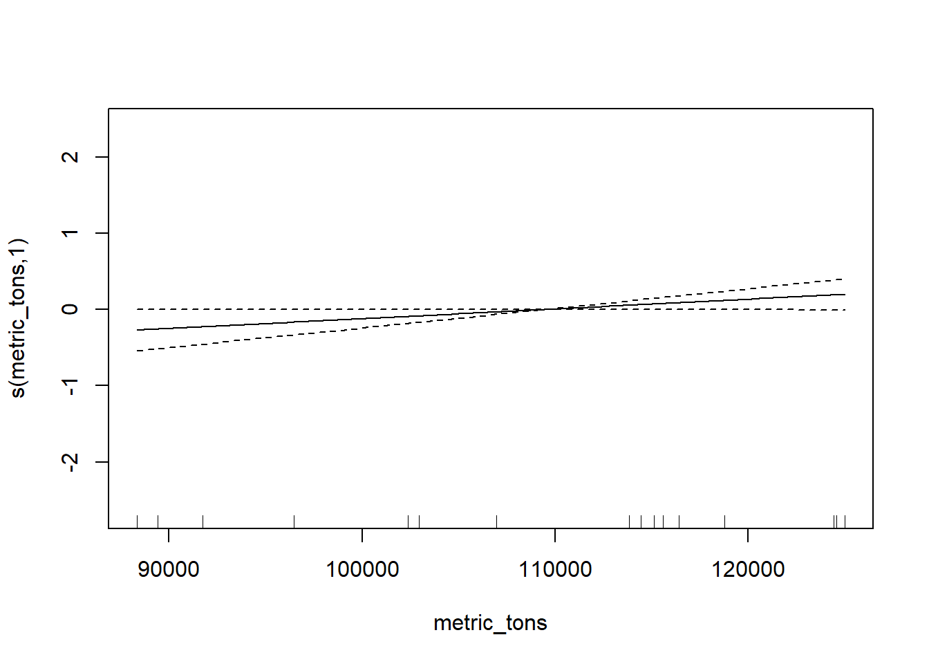
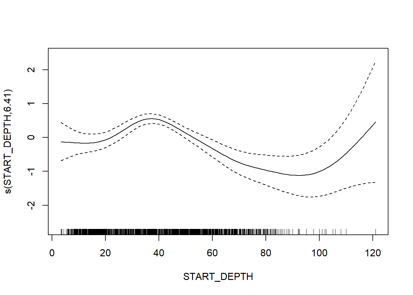
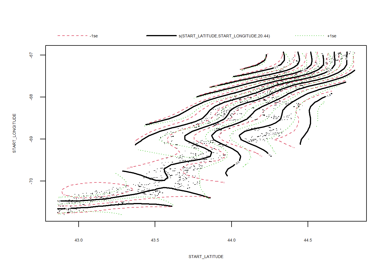
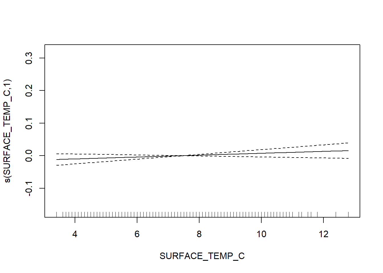
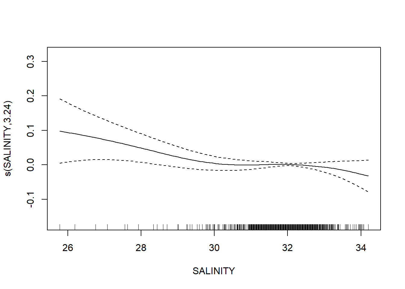
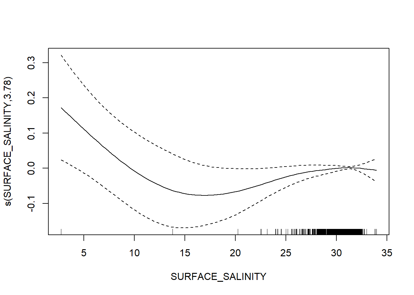
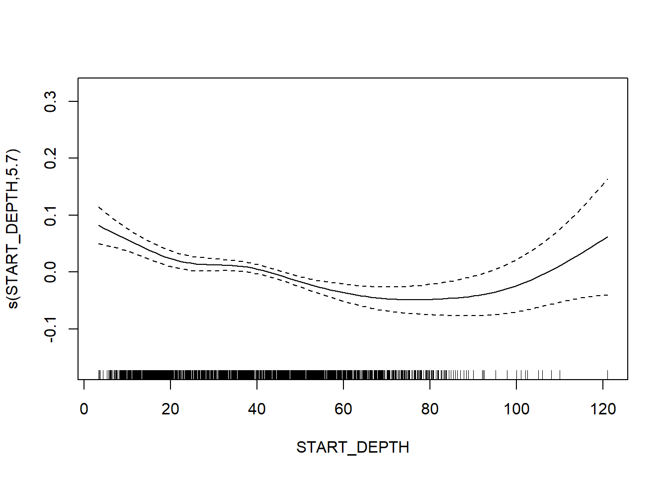
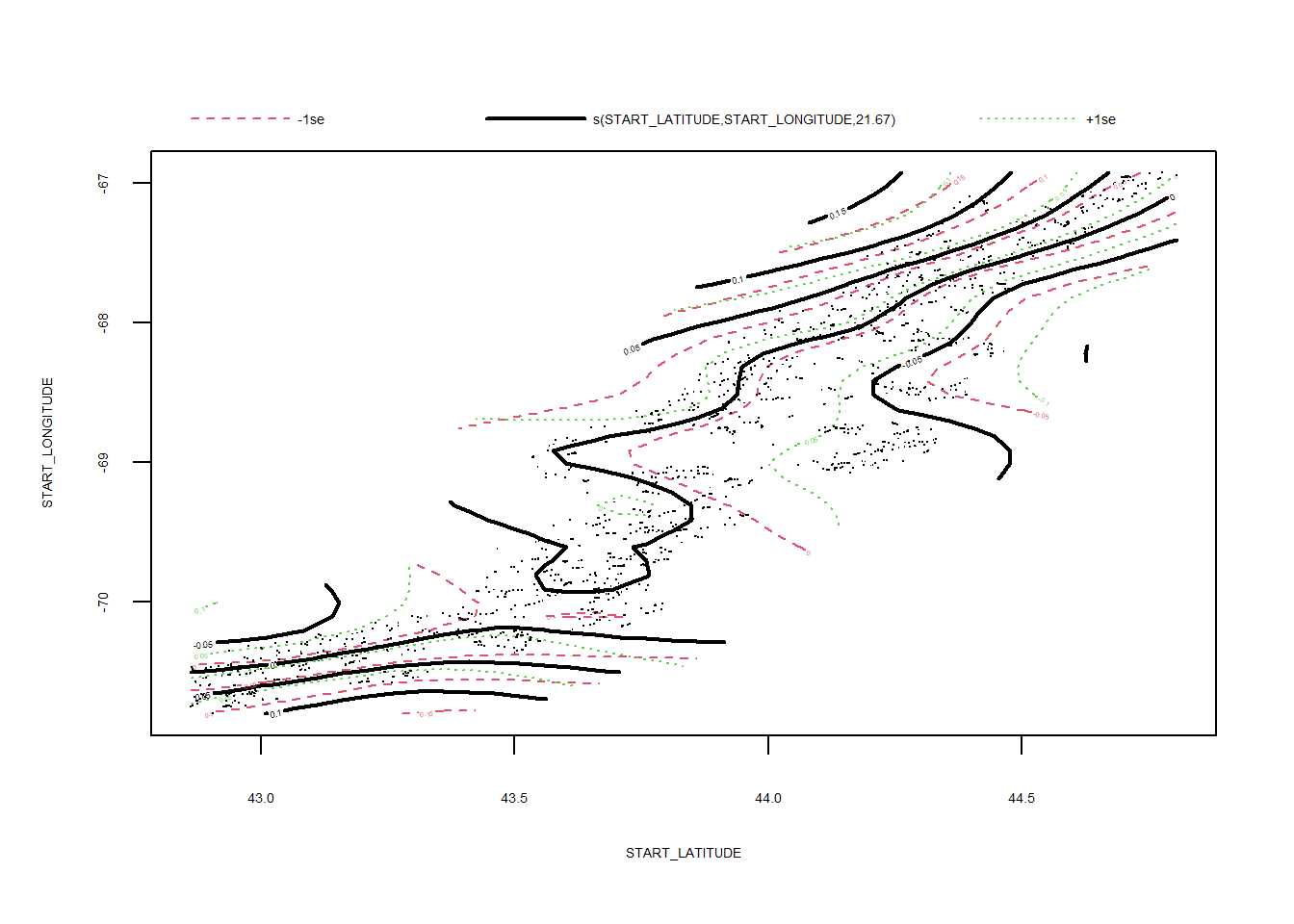
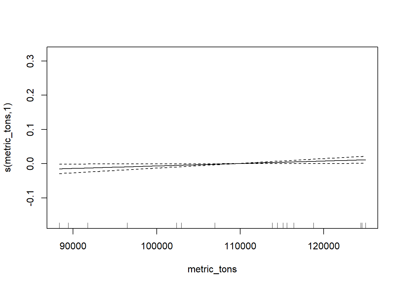
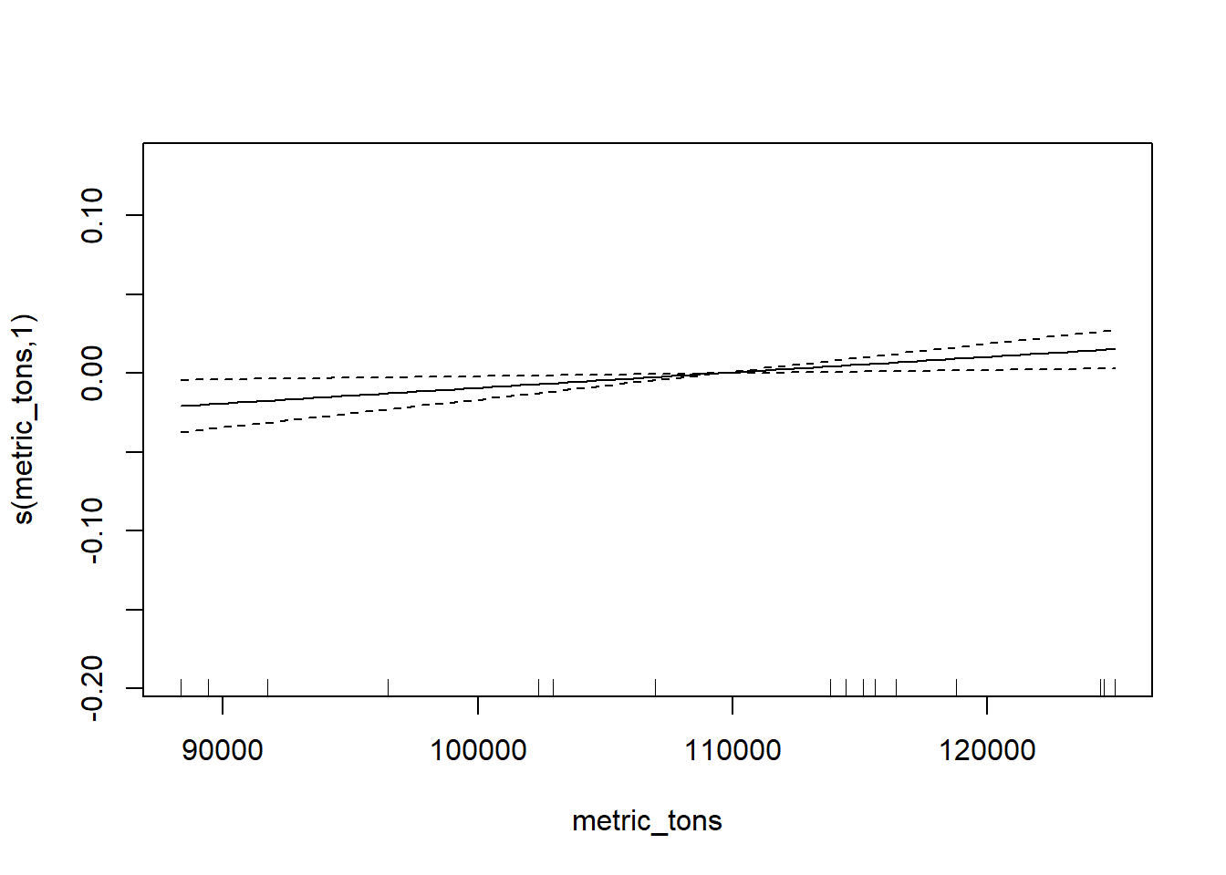
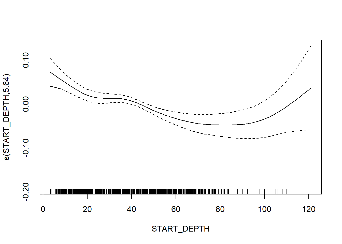
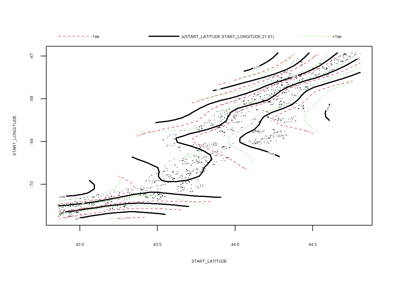
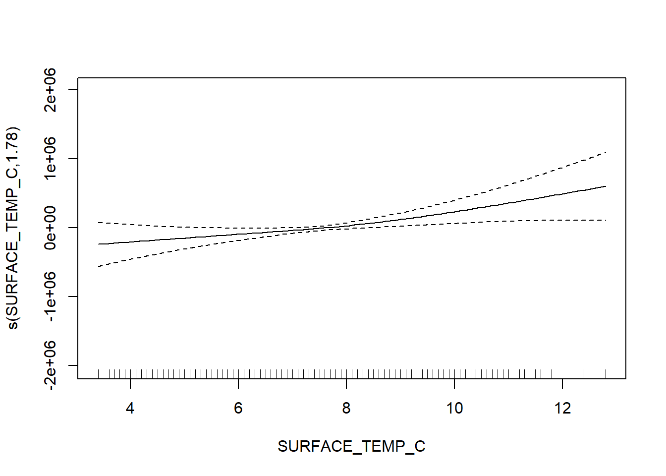
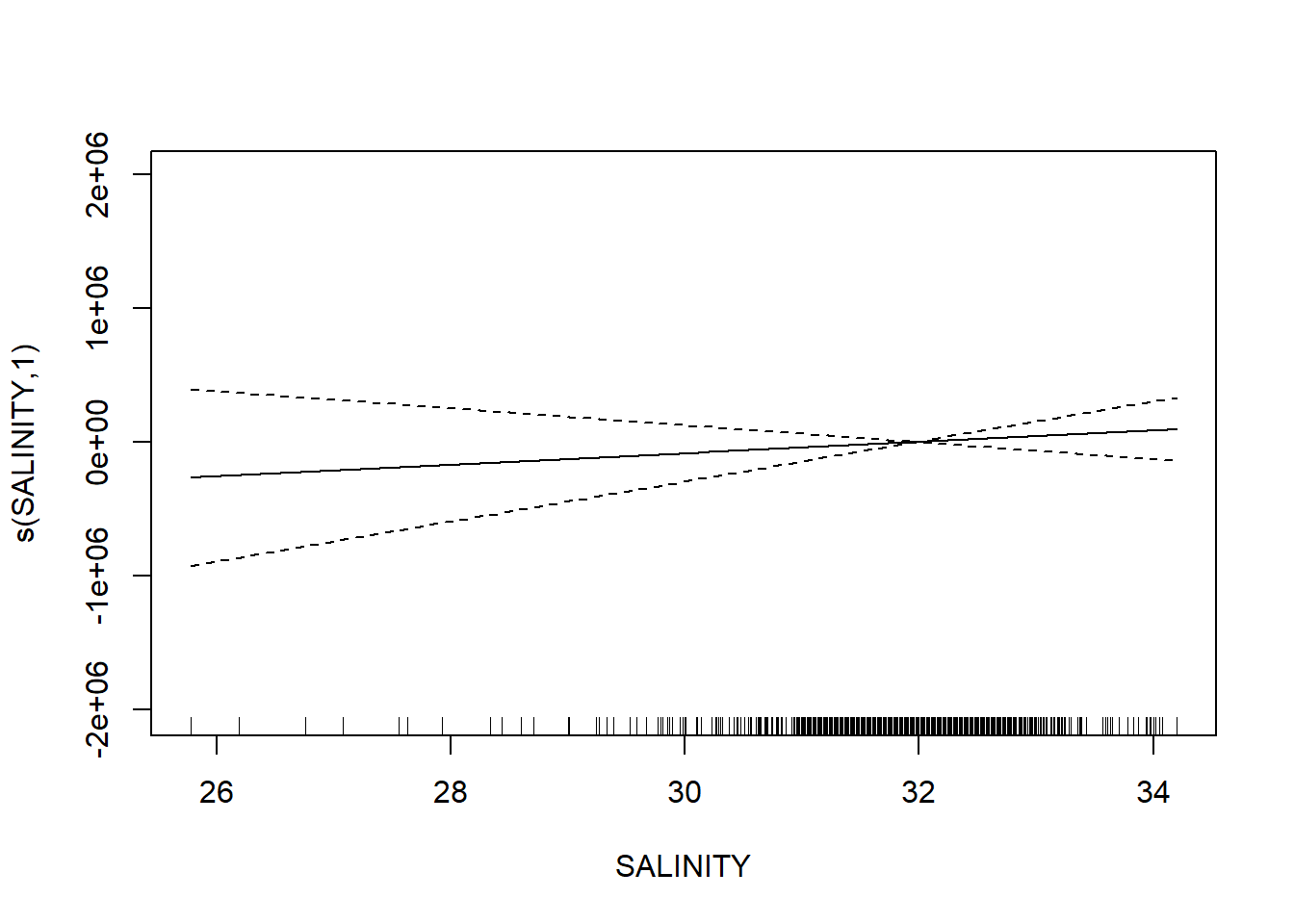
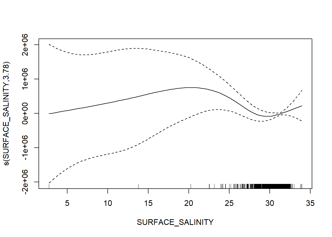
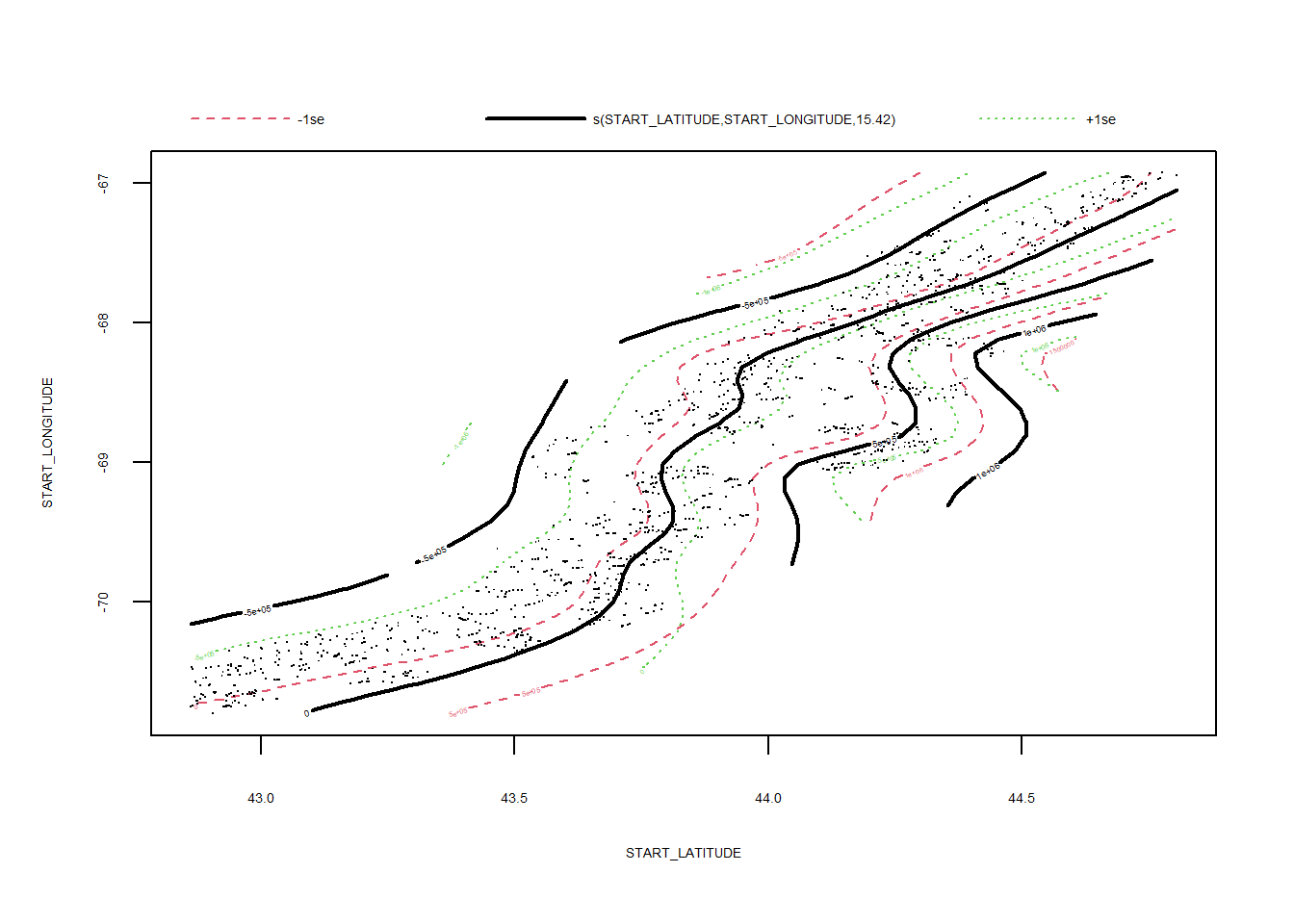
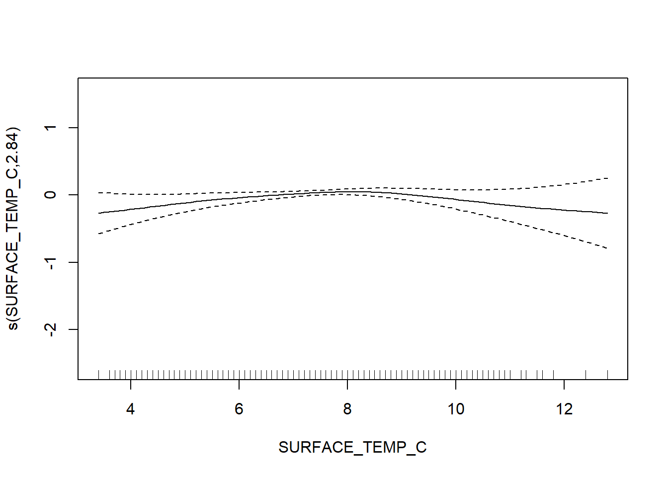
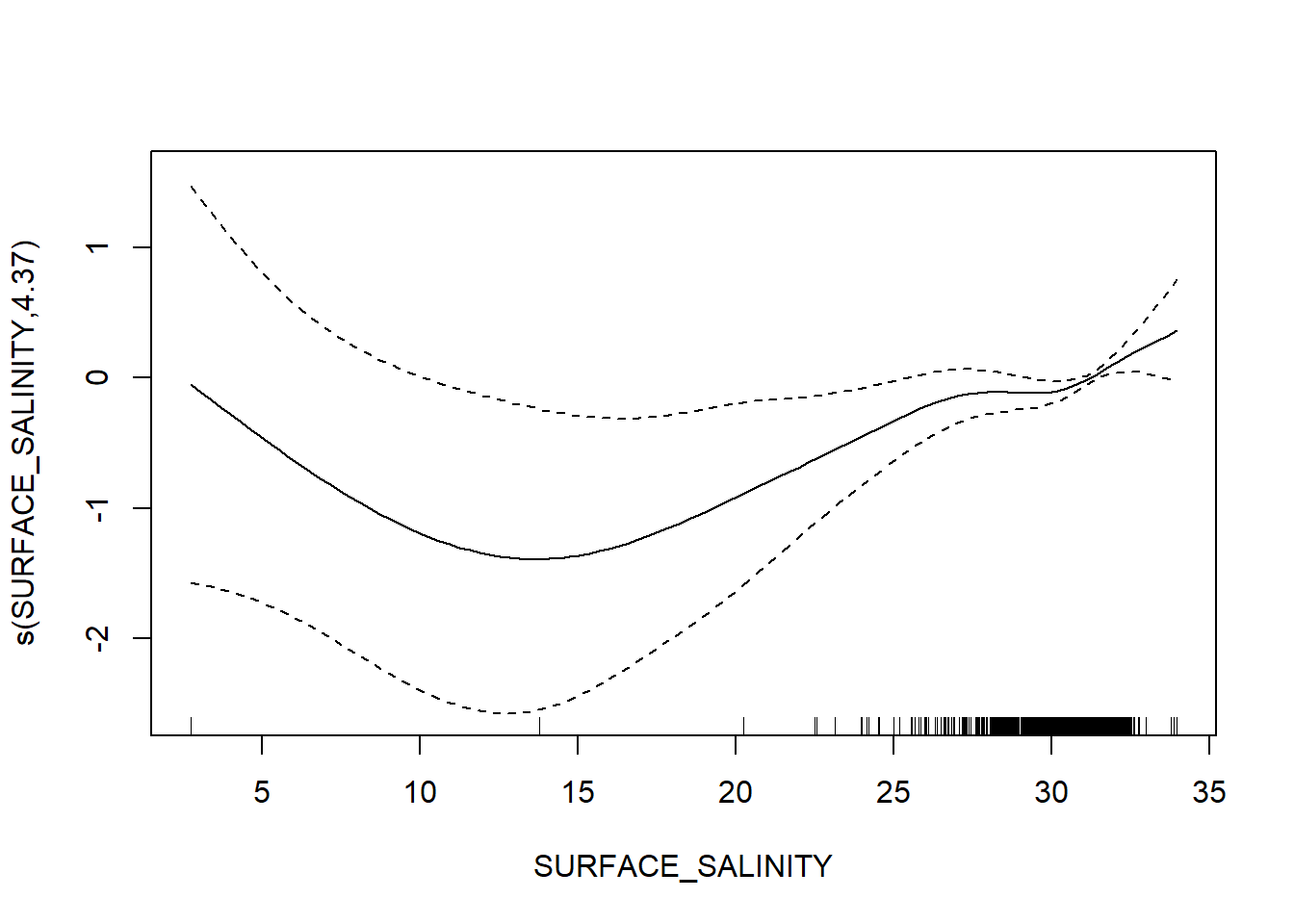
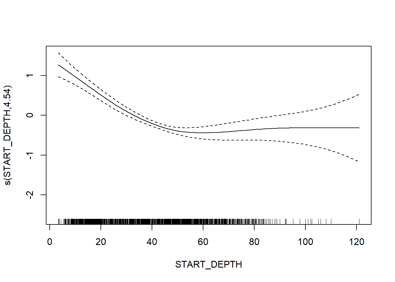
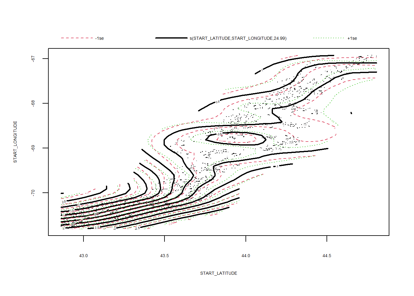
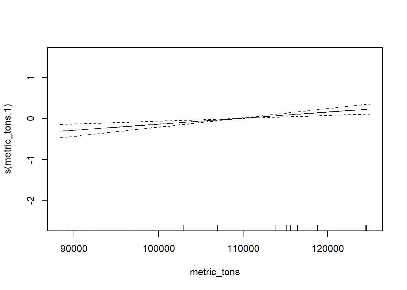
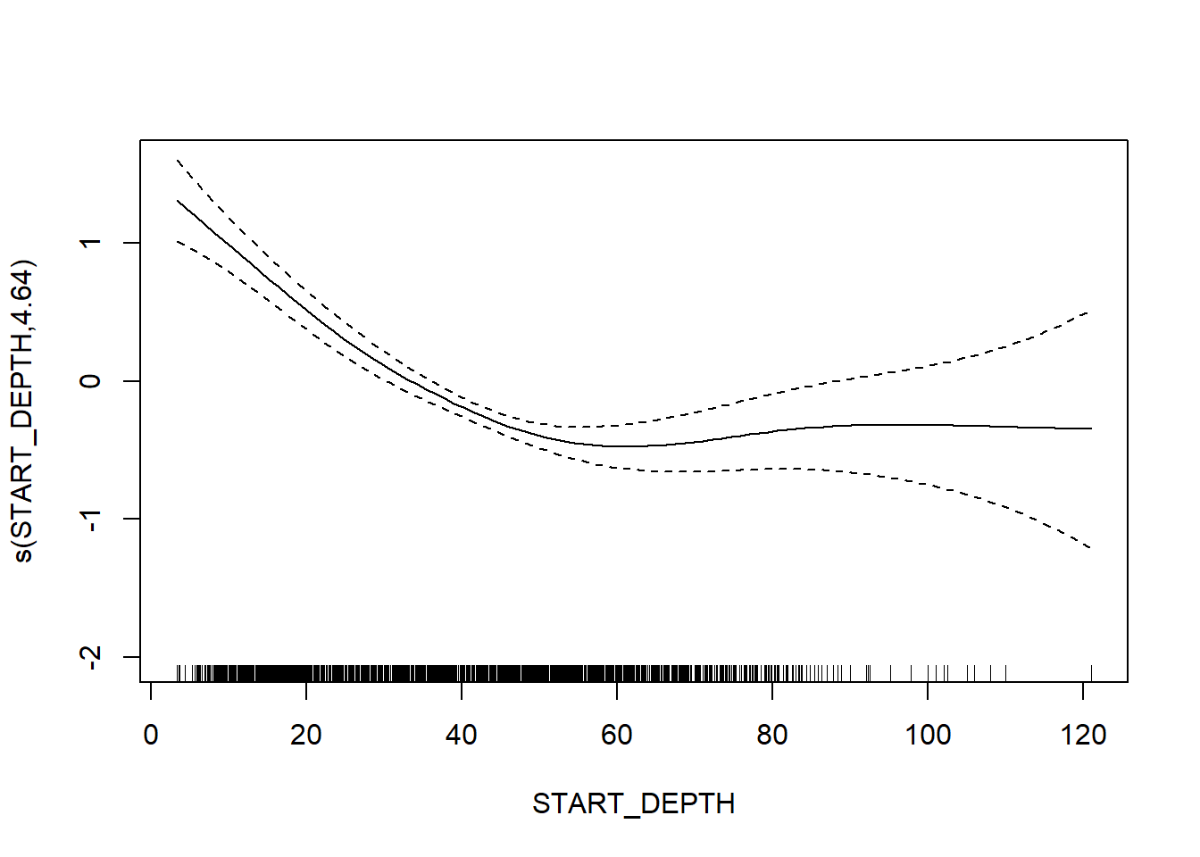
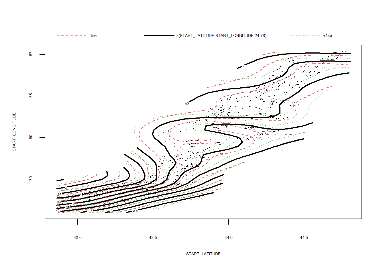
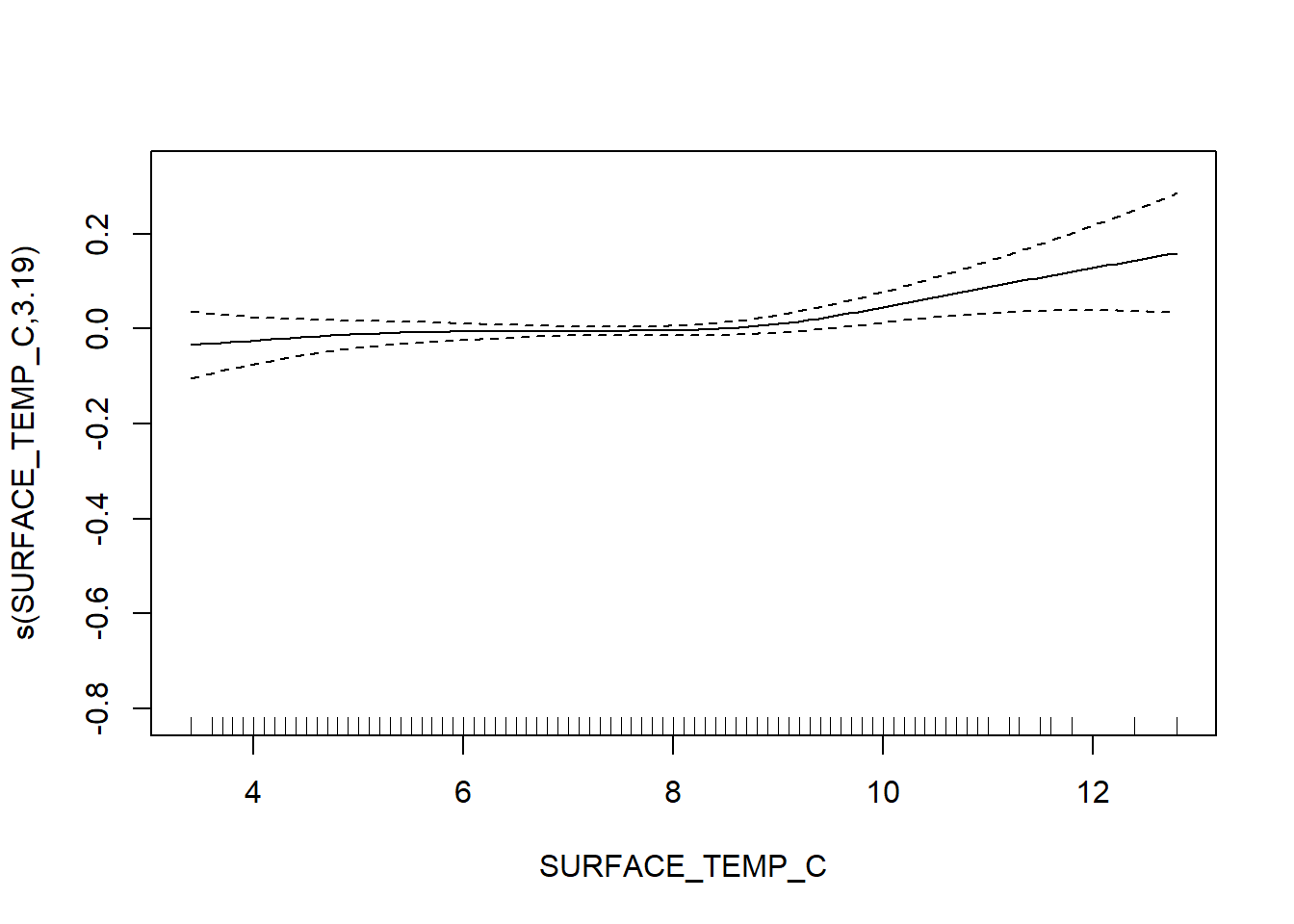
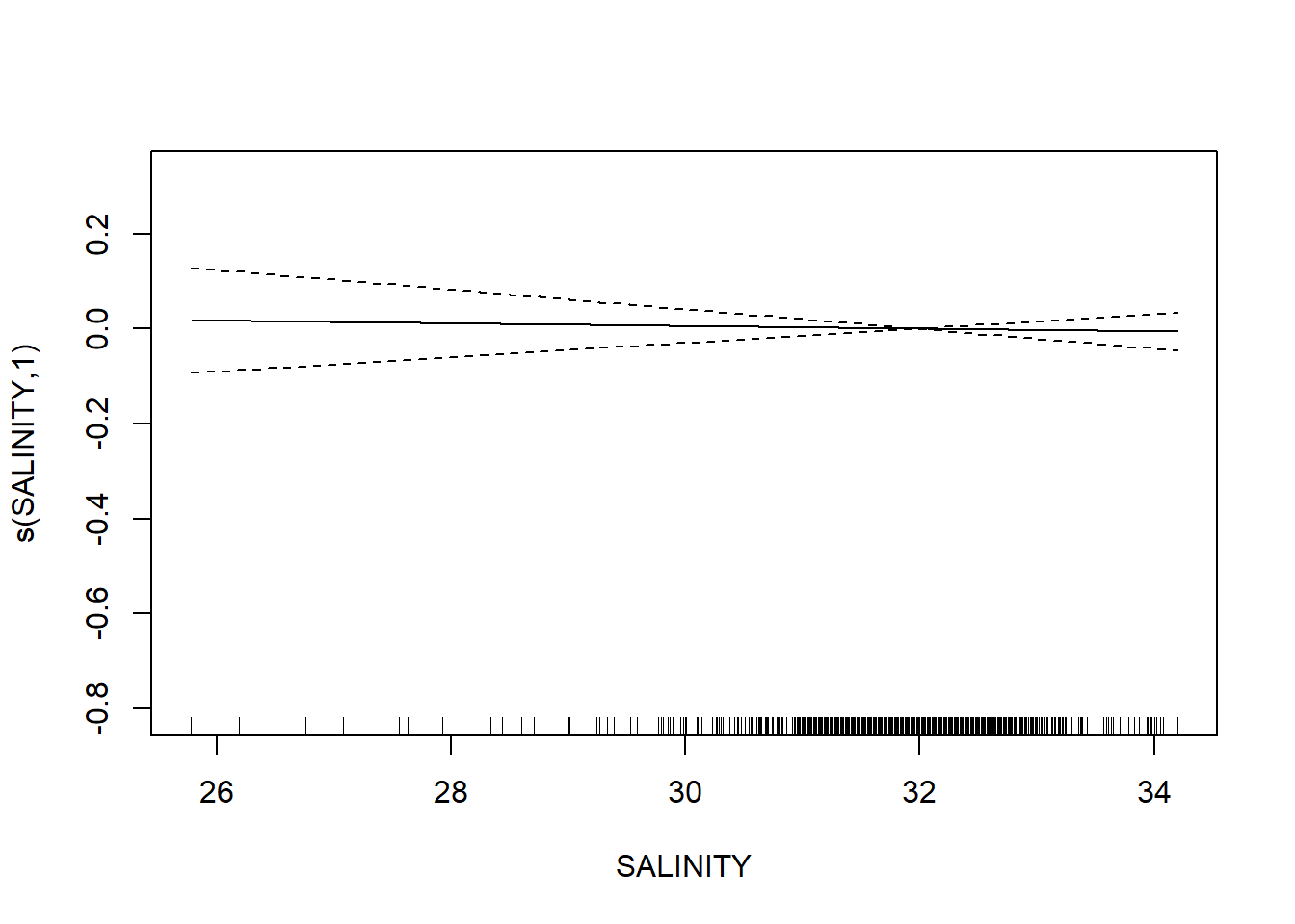
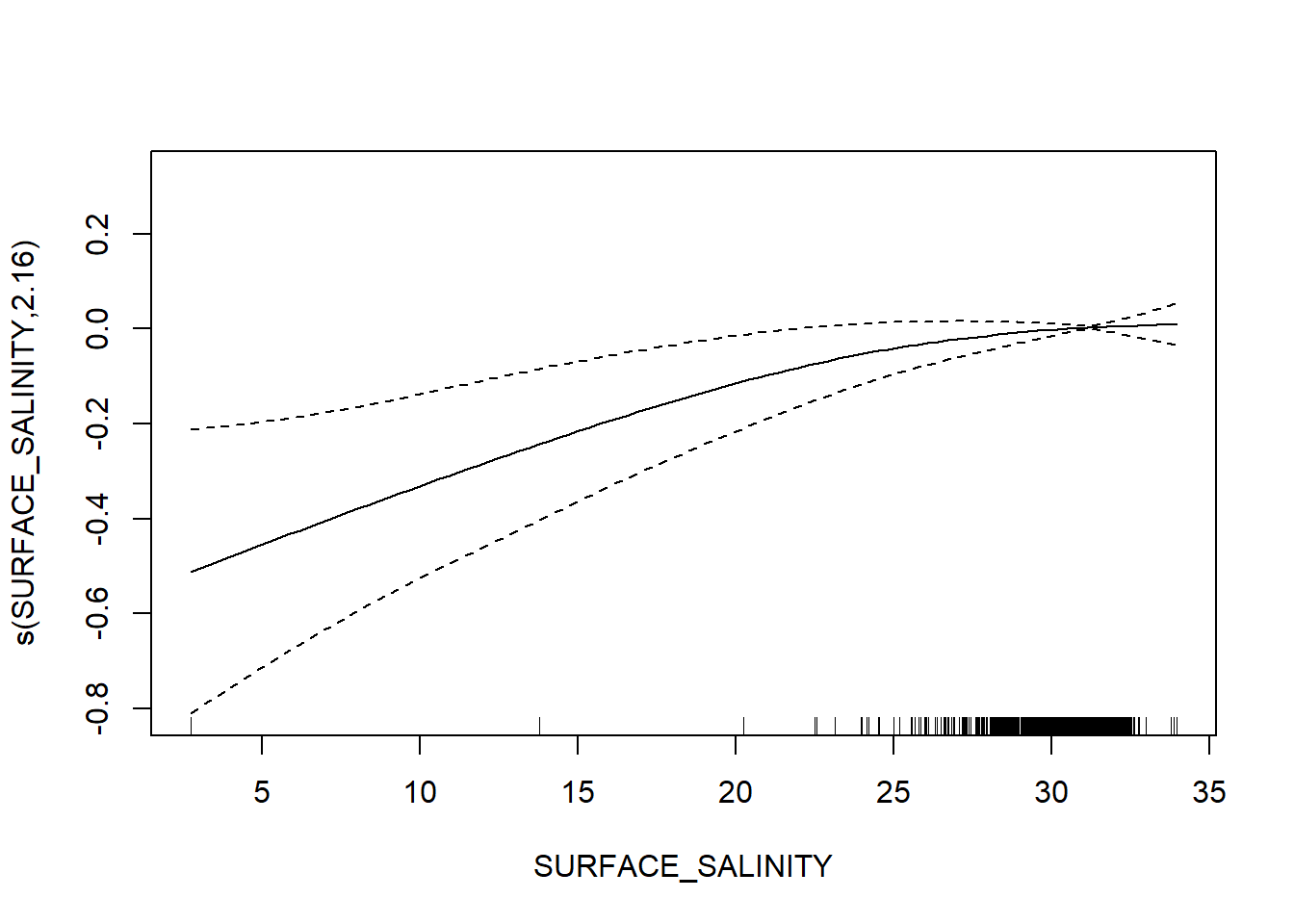
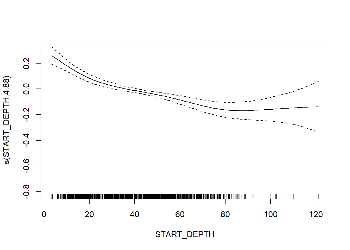
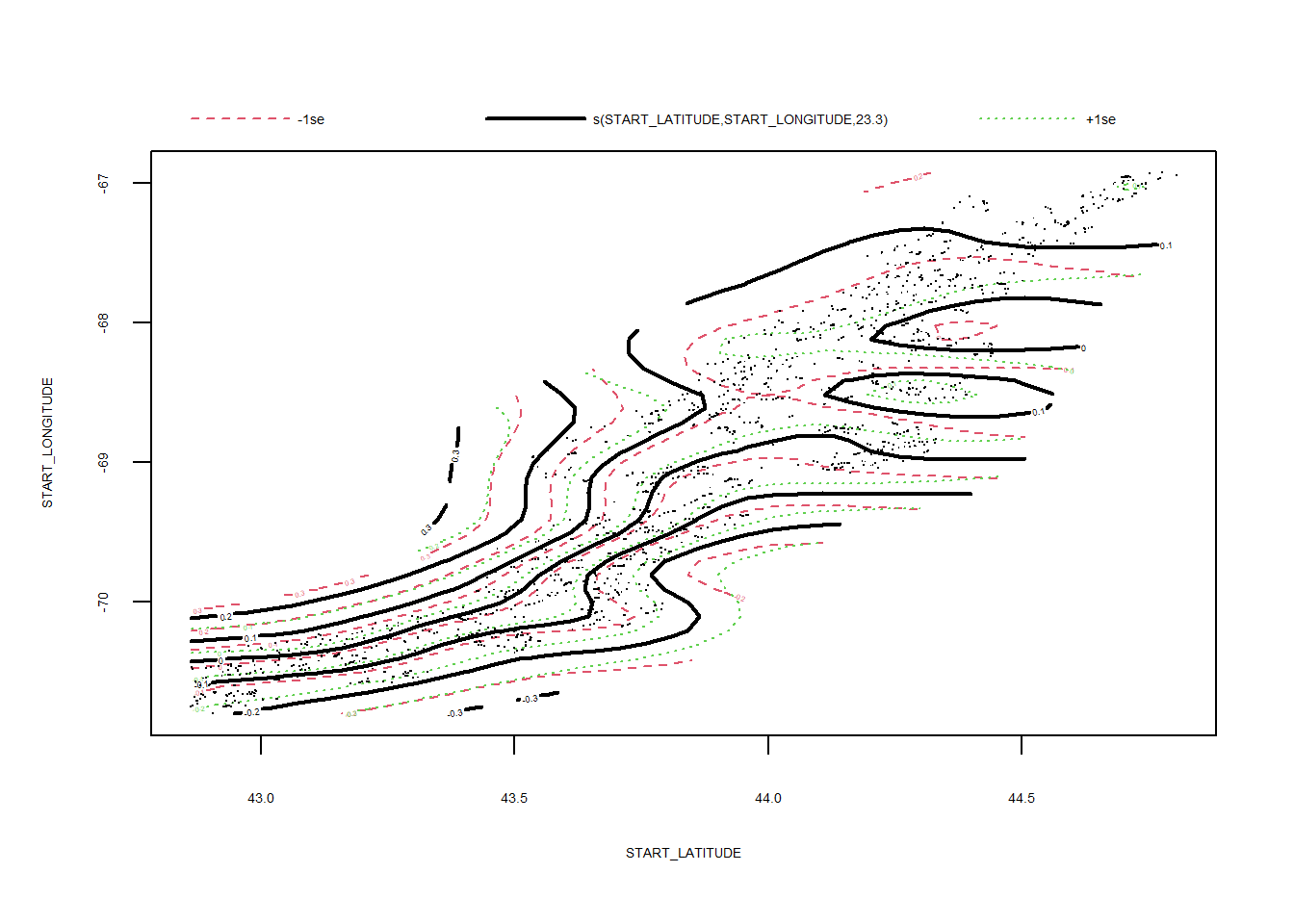
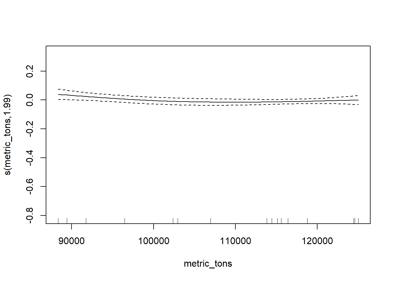
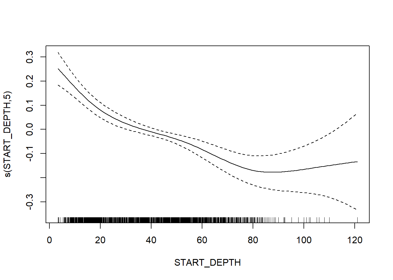
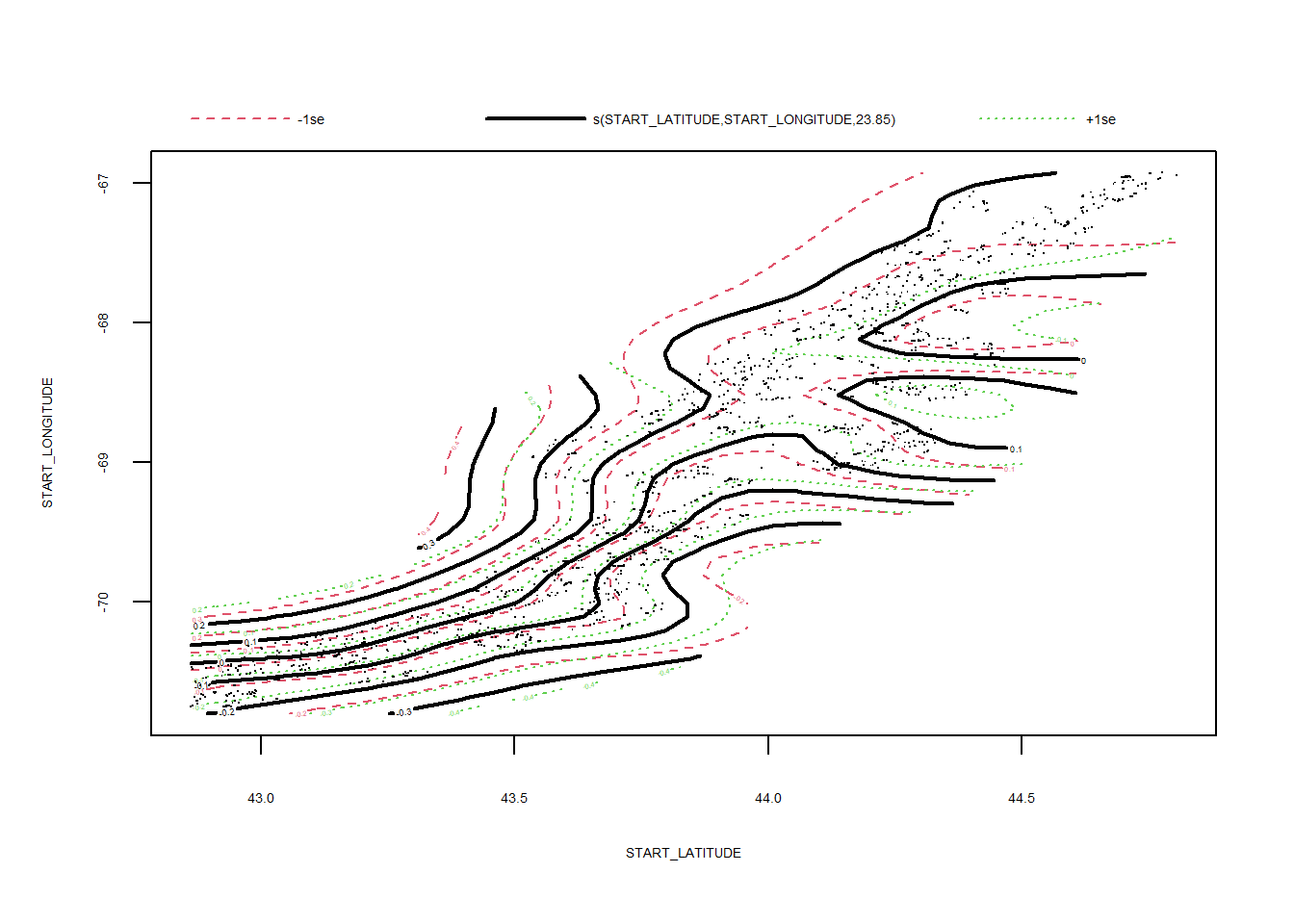
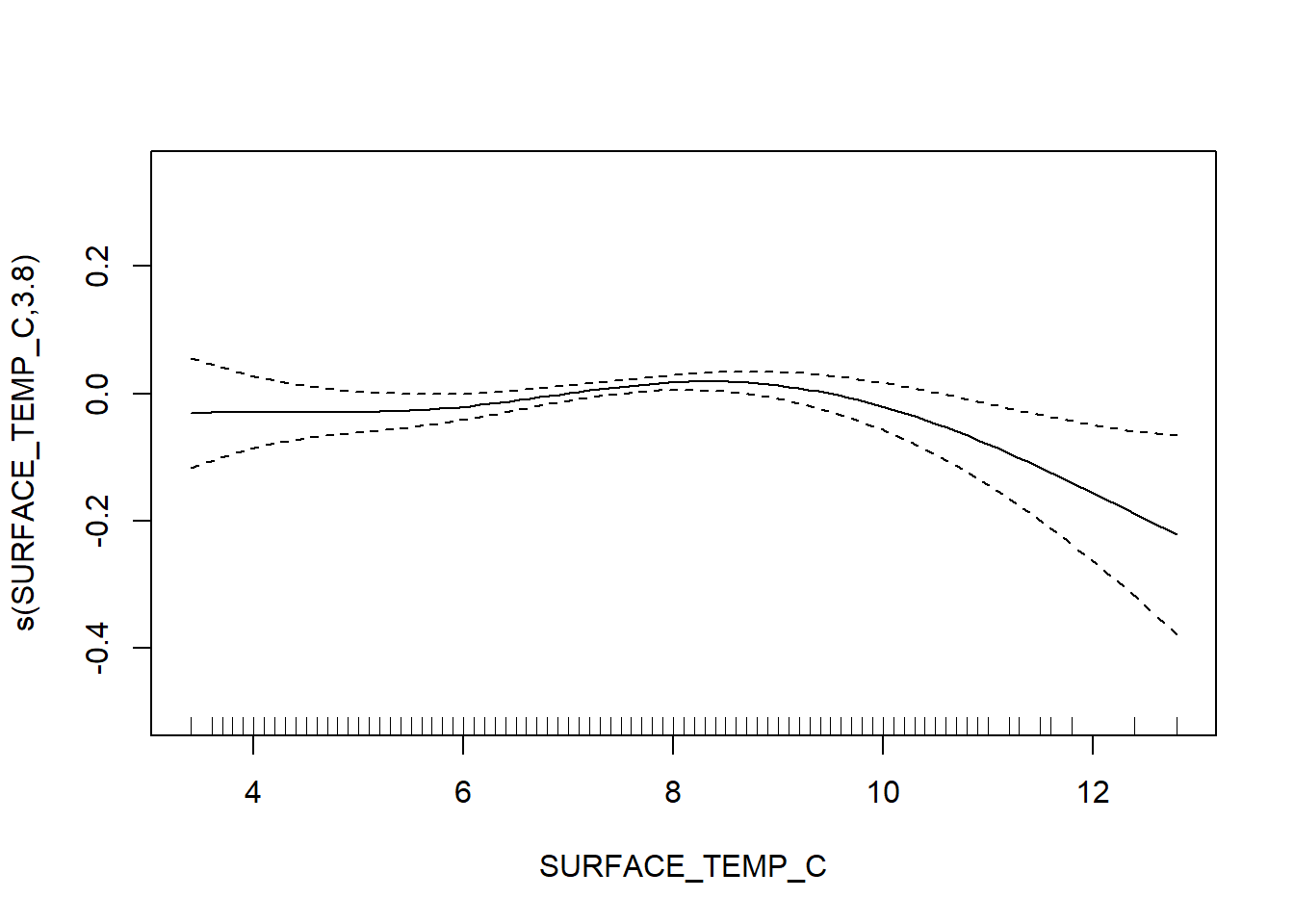
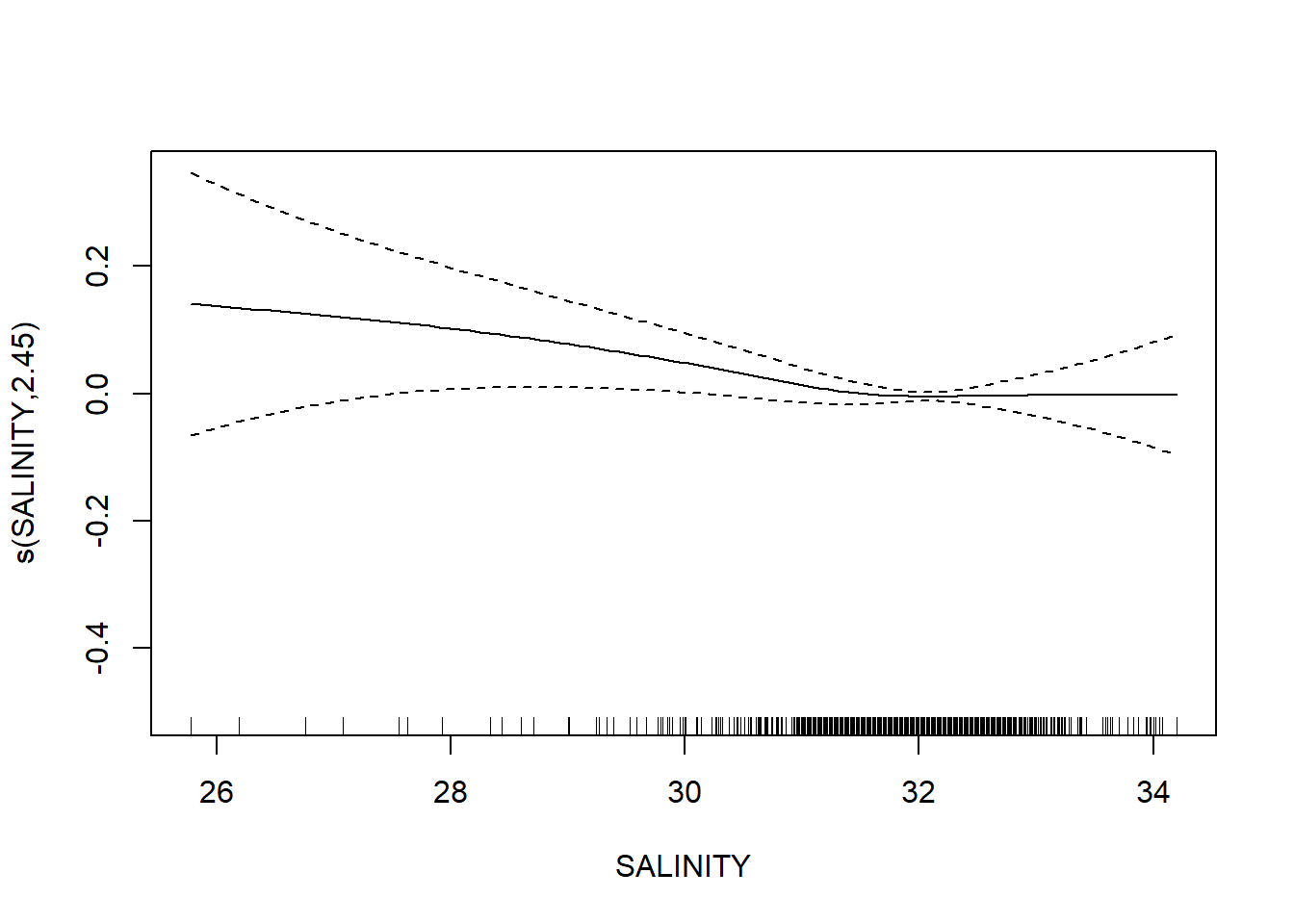
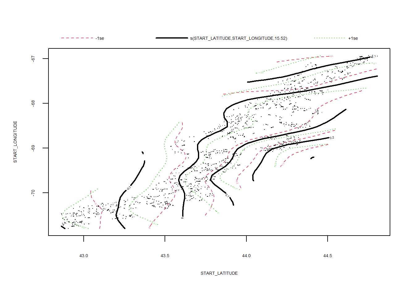
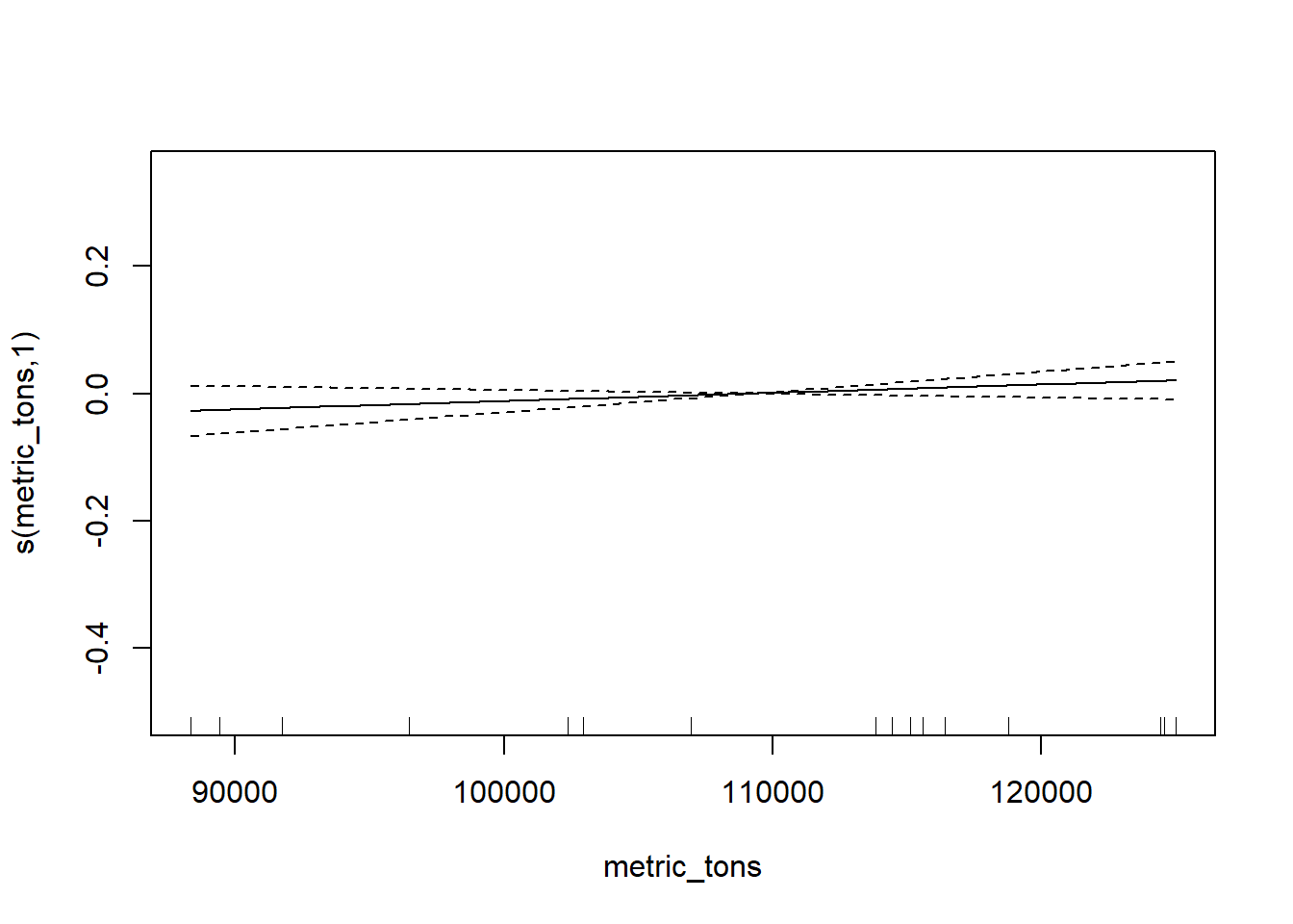
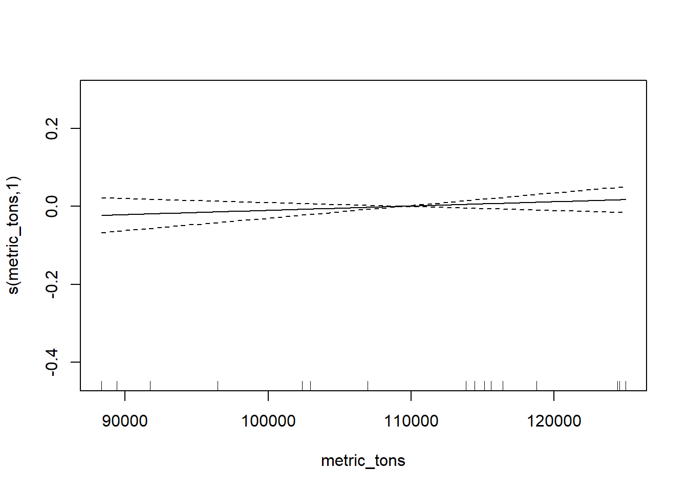
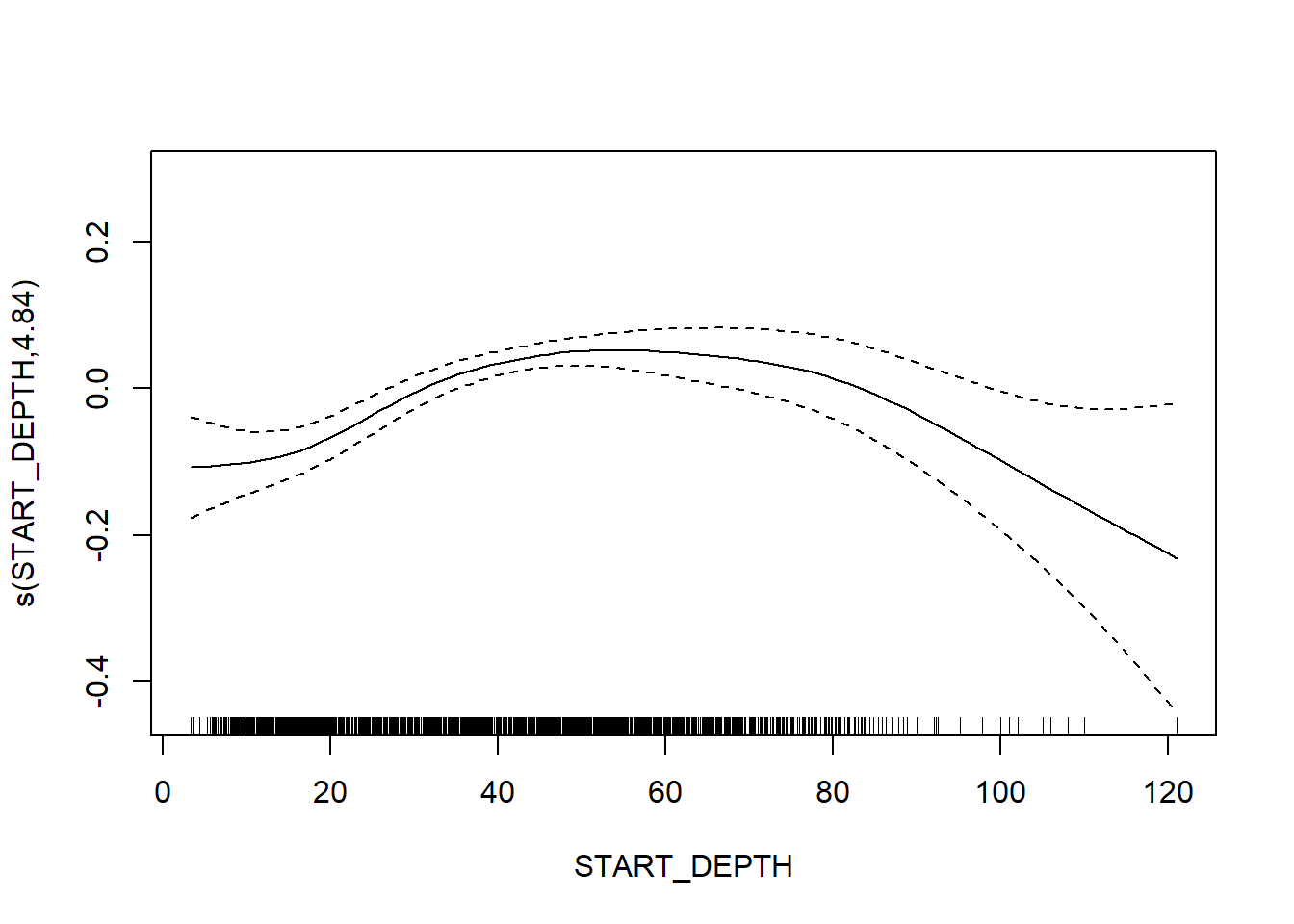
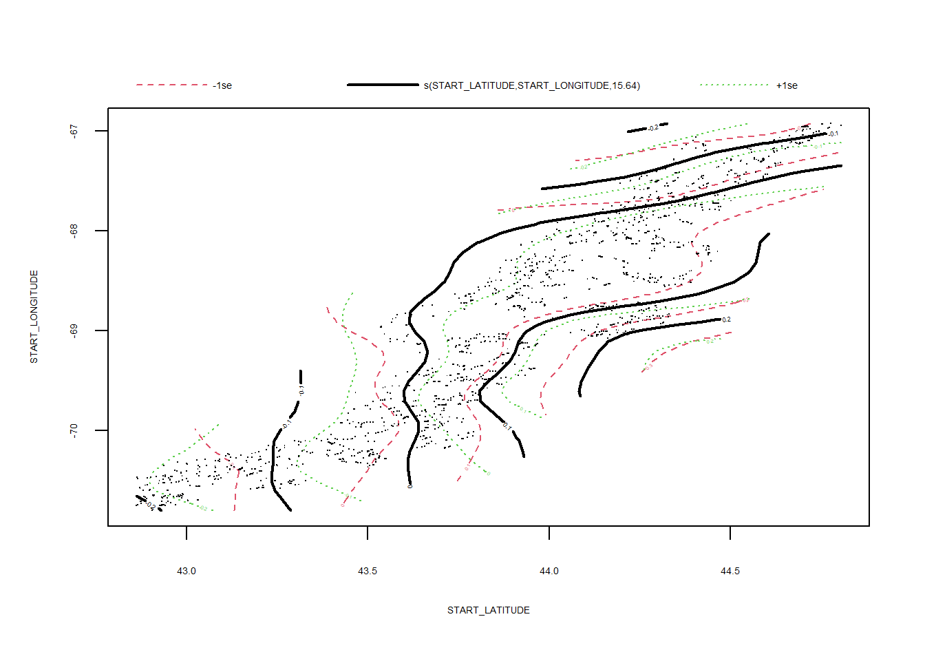
N_Fall_2 <- gamm4(N_species ~ s(WATER_TEMP_C) + s(SURFACE_TEMP_C) + s(SALINITY) + s(metric_tons) + s(SURFACE_SALINITY) + s(START_DEPTH) + s(START_LATITUDE, START_LONGITUDE), random = ~ (1|YEAR) , data = fall)
gam.check(N_Fall_2$gam)
##
## 'gamm' based fit - care required with interpretation.
## Checks based on working residuals may be misleading.
## Basis dimension (k) checking results. Low p-value (k-index<1) may
## indicate that k is too low, especially if edf is close to k'.
##
##                                      k'   edf k-index p-value
## s(WATER_TEMP_C)                    9.00  4.55    0.90  <2e-16 ***
## s(SURFACE_TEMP_C)                  9.00  1.00    0.91  <2e-16 ***
## s(SALINITY)                        9.00  1.00    0.96   0.100 .
## s(metric_tons)                     9.00  1.65    0.81  <2e-16 ***
## s(SURFACE_SALINITY)                9.00  1.80    0.93   0.005 **
## s(START_DEPTH)                     9.00  5.84    0.96   0.105
## s(START_LATITUDE,START_LONGITUDE) 29.00 14.99    0.93   0.005 **
## ---
## Signif. codes:  0 '***' 0.001 '**' 0.01 '*' 0.05 '.' 0.1 ' ' 1
# plot(resid(N_Fall_2$gam))
# abline(h = 0)
#mean(resid(N_Fall_2$gam)^2)
#5 significant trend?
# interpretting results
summary(N_Fall_2$gam) # importance of terms ##
## Family: gaussian
## Link function: identity
##
## Formula:
## N_species ~ s(WATER_TEMP_C) + s(SURFACE_TEMP_C) + s(SALINITY) +
## s(metric_tons) + s(SURFACE_SALINITY) + s(START_DEPTH) + s(START_LATITUDE,
## START_LONGITUDE)
##
## Parametric coefficients:
## Estimate Std. Error t value Pr(>|t|)
## (Intercept) 21.2828 0.2413 88.2 <2e-16 ***
## ---
## Signif. codes: 0 '***' 0.001 '**' 0.01 '*' 0.05 '.' 0.1 ' ' 1
##
## Approximate significance of smooth terms:
## edf Ref.df F p-value
## s(WATER_TEMP_C) 4.552 4.552 5.088 0.000254 ***
## s(SURFACE_TEMP_C) 1.000 1.000 0.069 0.793097
## s(SALINITY) 1.000 1.000 3.567 0.059176 .
## s(metric_tons) 1.648 1.648 5.992 0.003389 **
## s(SURFACE_SALINITY) 1.803 1.803 0.860 0.314348
## s(START_DEPTH) 5.843 5.843 31.320 < 2e-16 ***
## s(START_LATITUDE,START_LONGITUDE) 14.986 14.986 4.282 < 2e-16 ***
## ---
## Signif. codes: 0 '***' 0.001 '**' 0.01 '*' 0.05 '.' 0.1 ' ' 1
##
## R-sq.(adj) = 0.419
## lmer.REML = 6967.2 Scale est. = 11.215 n = 1309print(N_Fall_2$gam) # edf; higher = more complex splines ##
## Family: gaussian
## Link function: identity
##
## Formula:
## N_species ~ s(WATER_TEMP_C) + s(SURFACE_TEMP_C) + s(SALINITY) +
## s(metric_tons) + s(SURFACE_SALINITY) + s(START_DEPTH) + s(START_LATITUDE,
## START_LONGITUDE)
##
## Estimated degrees of freedom:
## 4.55 1.00 1.00 1.65 1.80 5.84 14.99
## total = 31.83
##
## lmer.REML score: 6967.207#confint(N_Fall_2$gam)
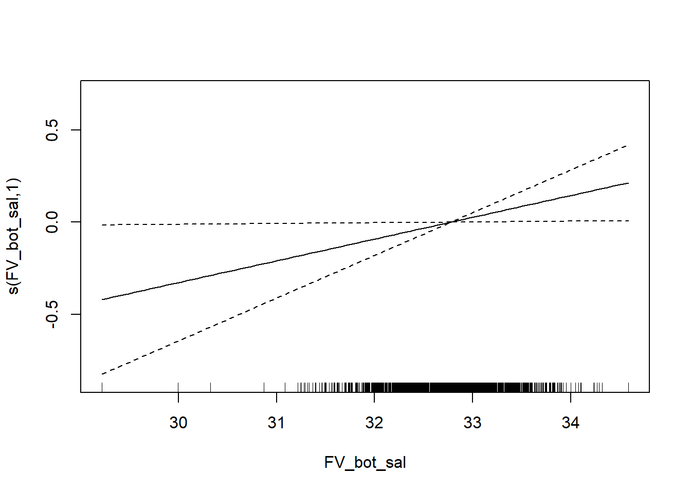
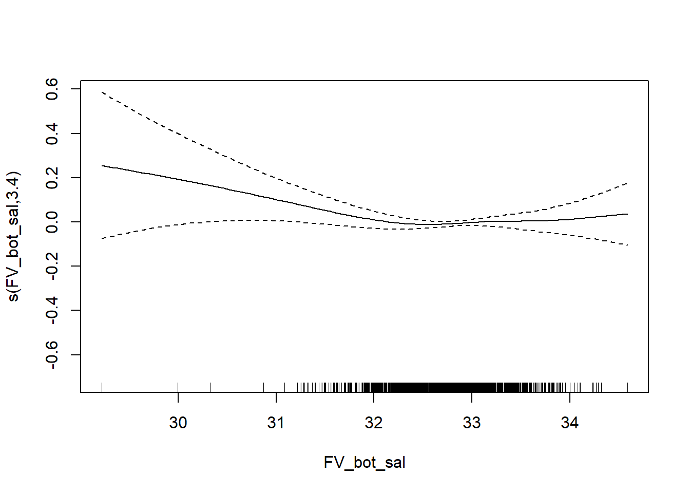
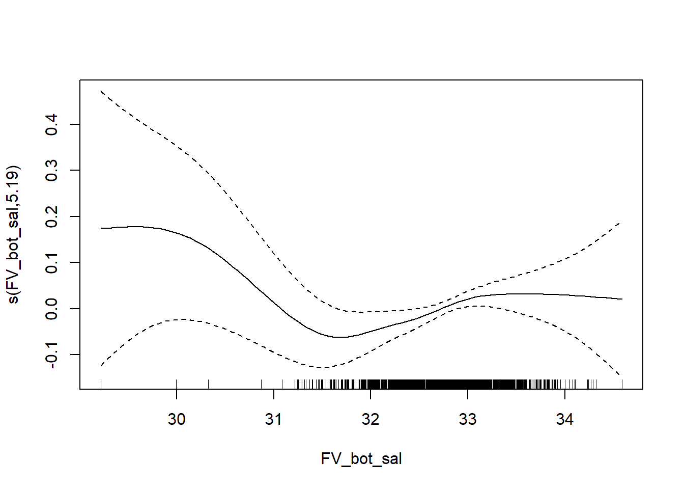
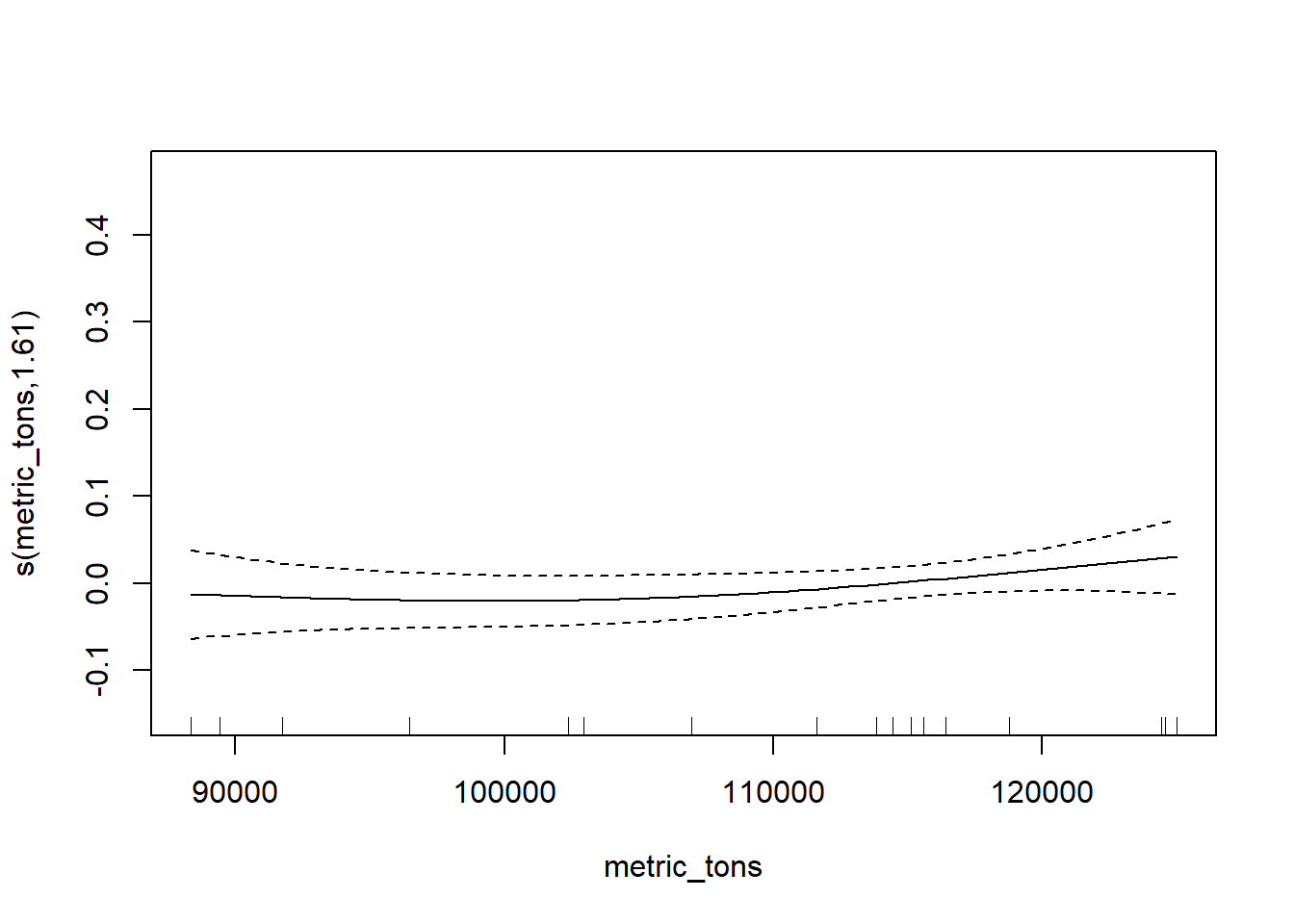
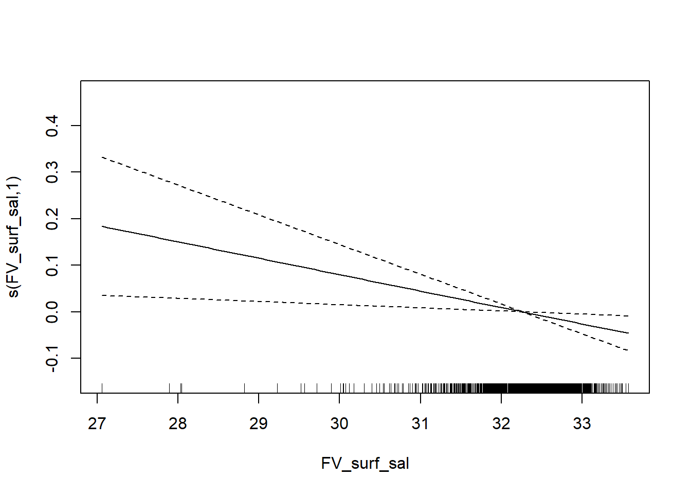
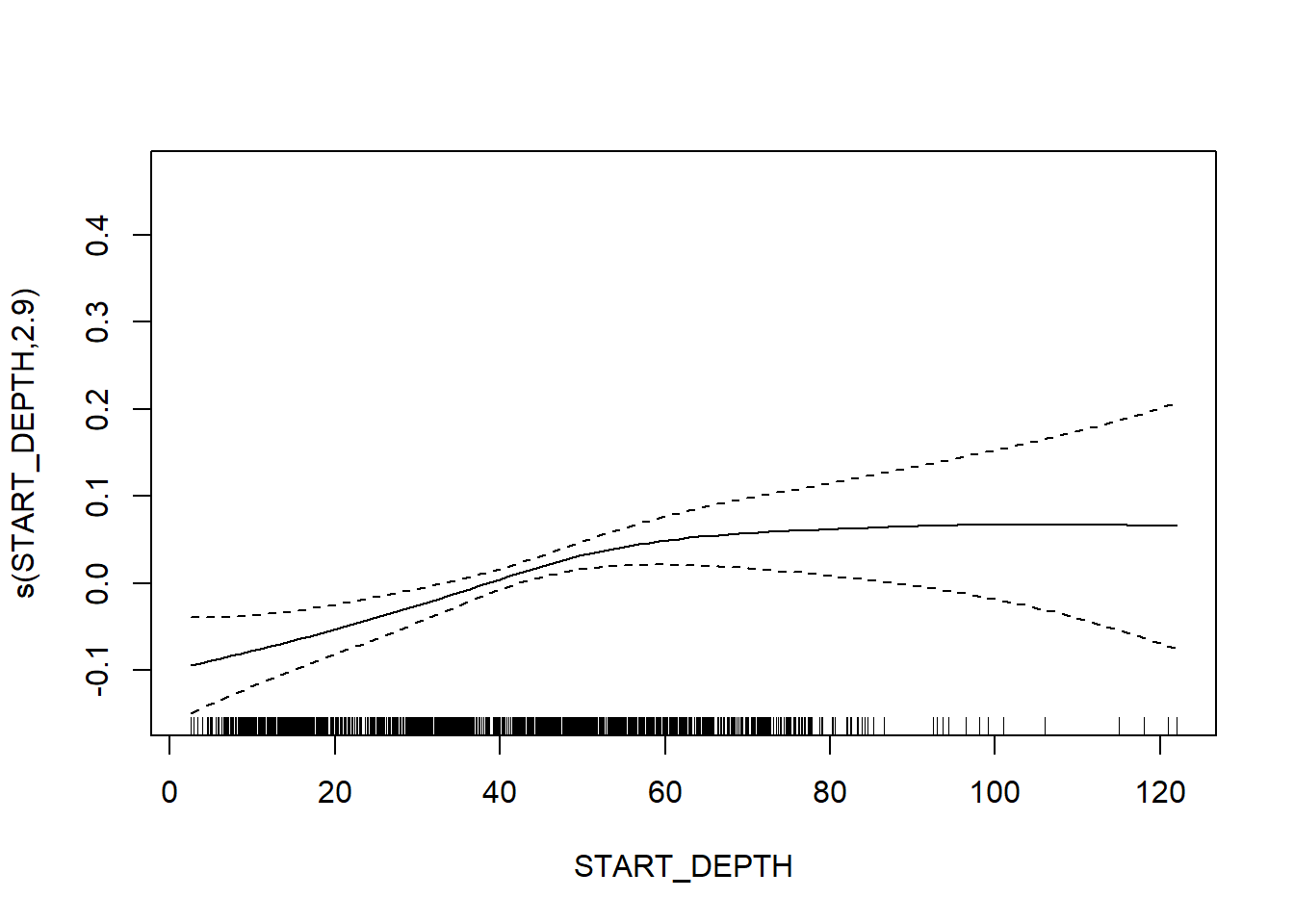
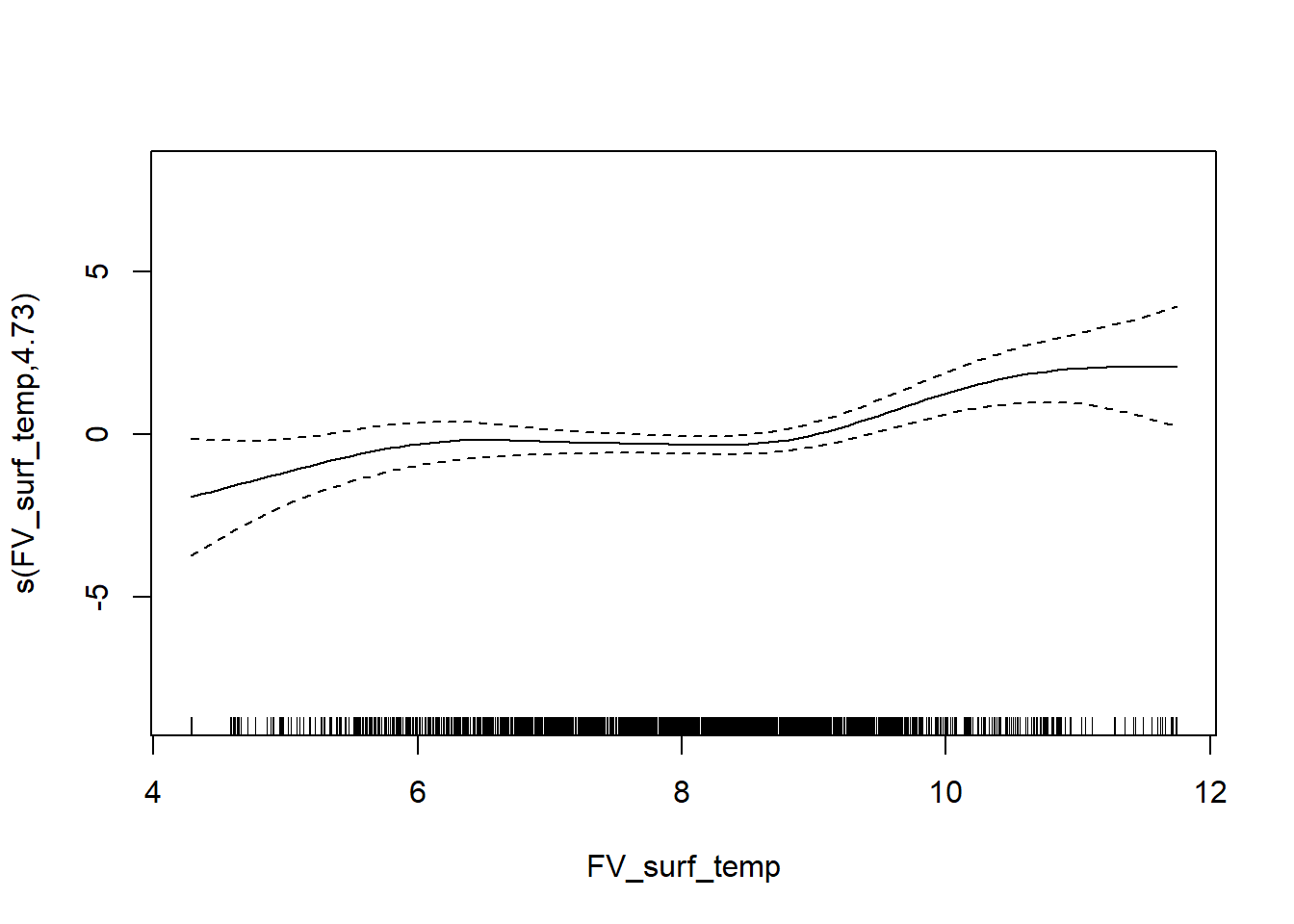
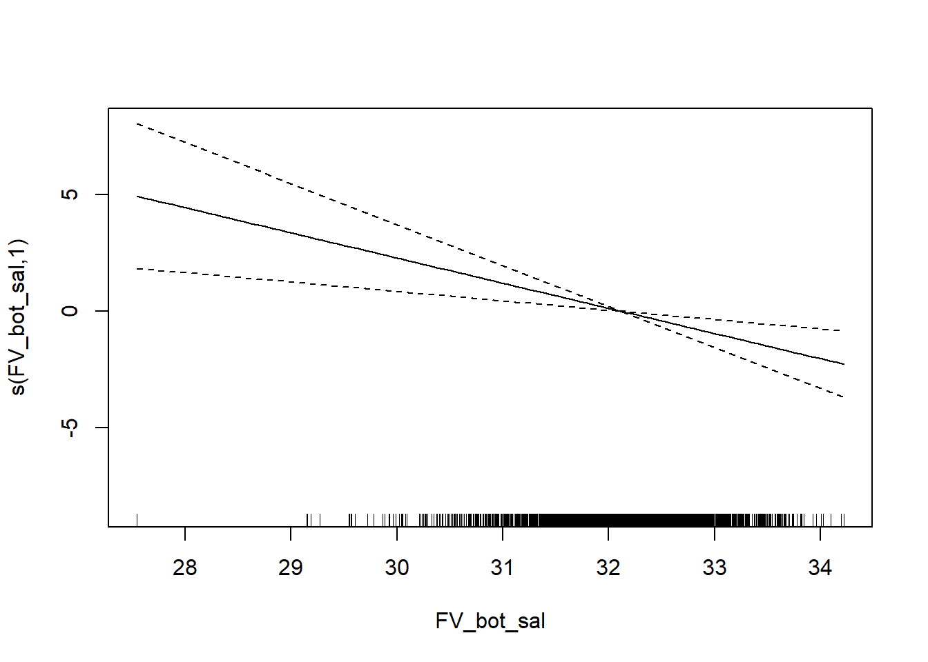
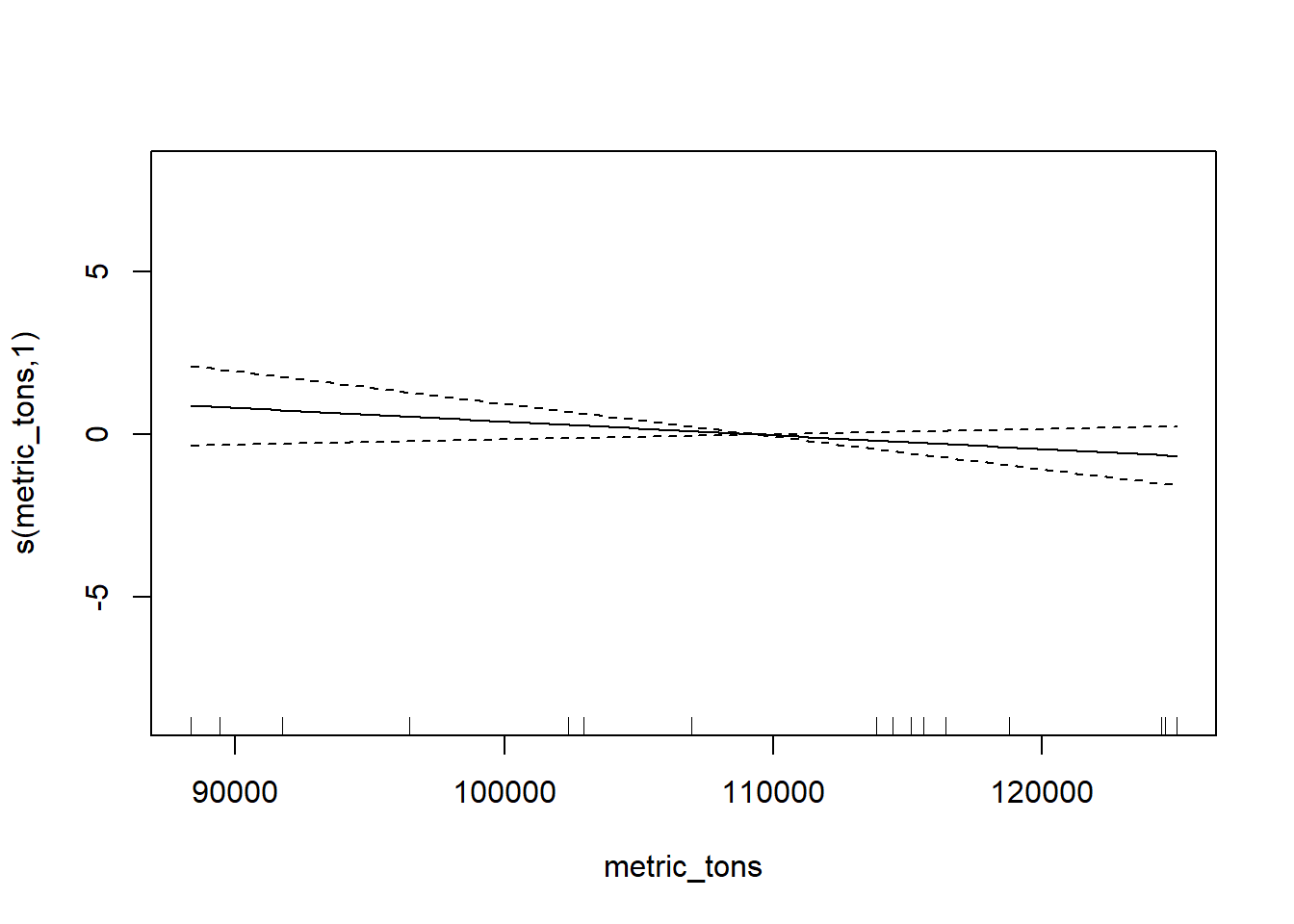
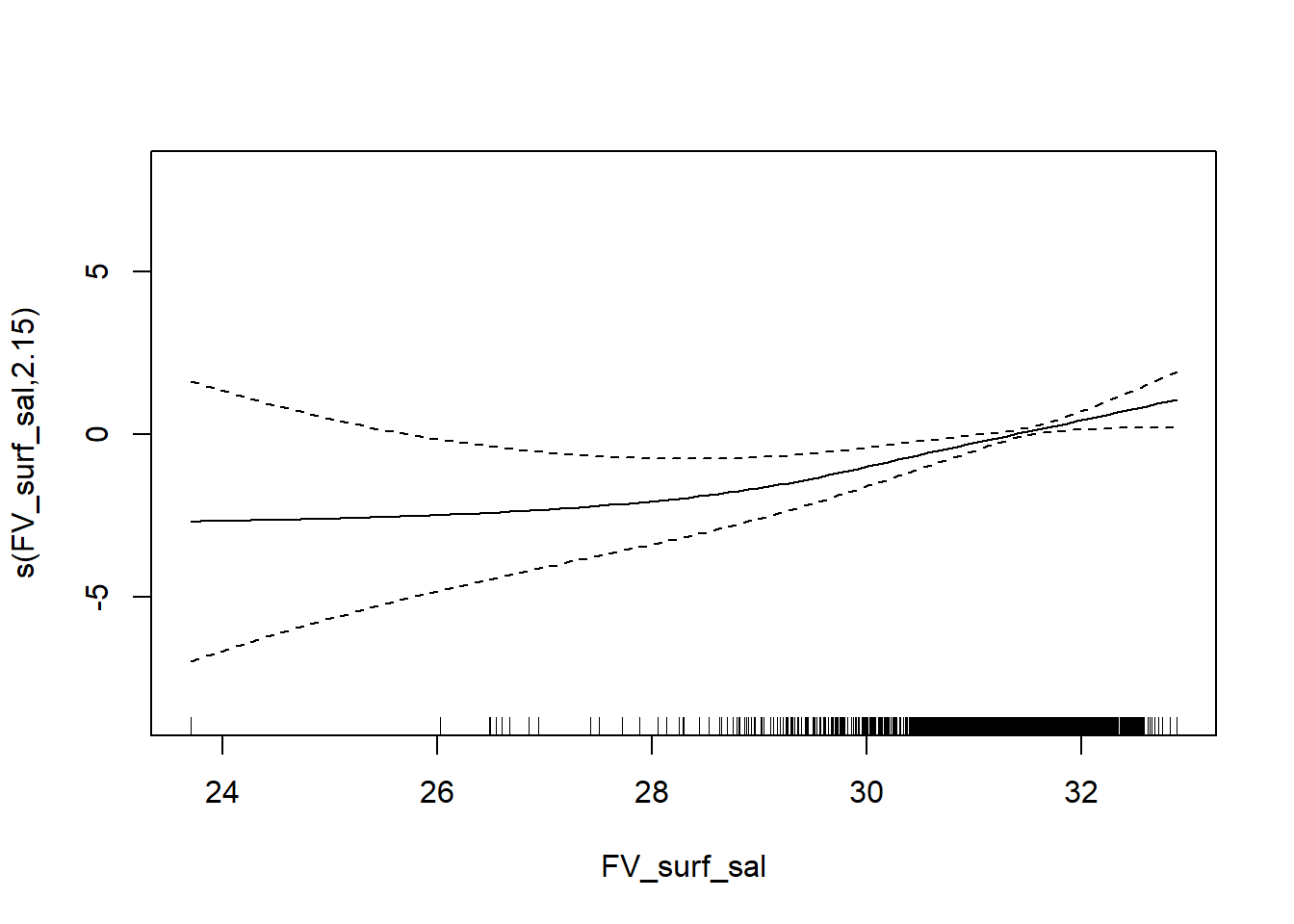
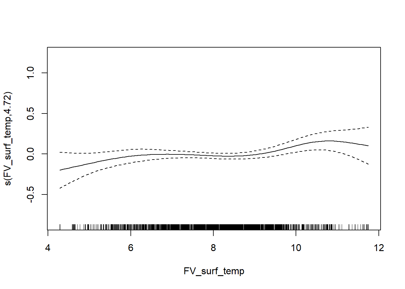
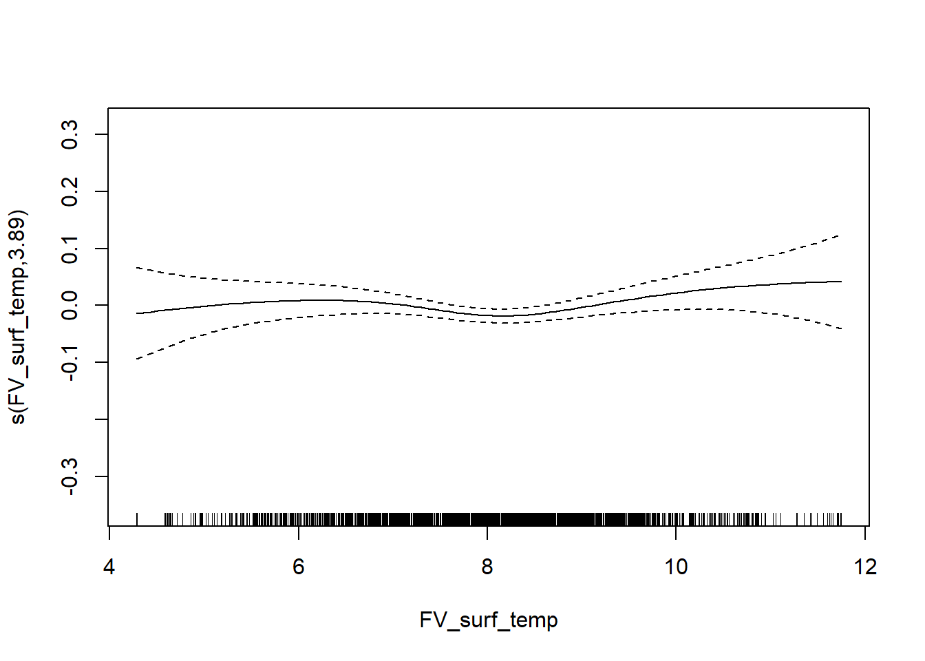
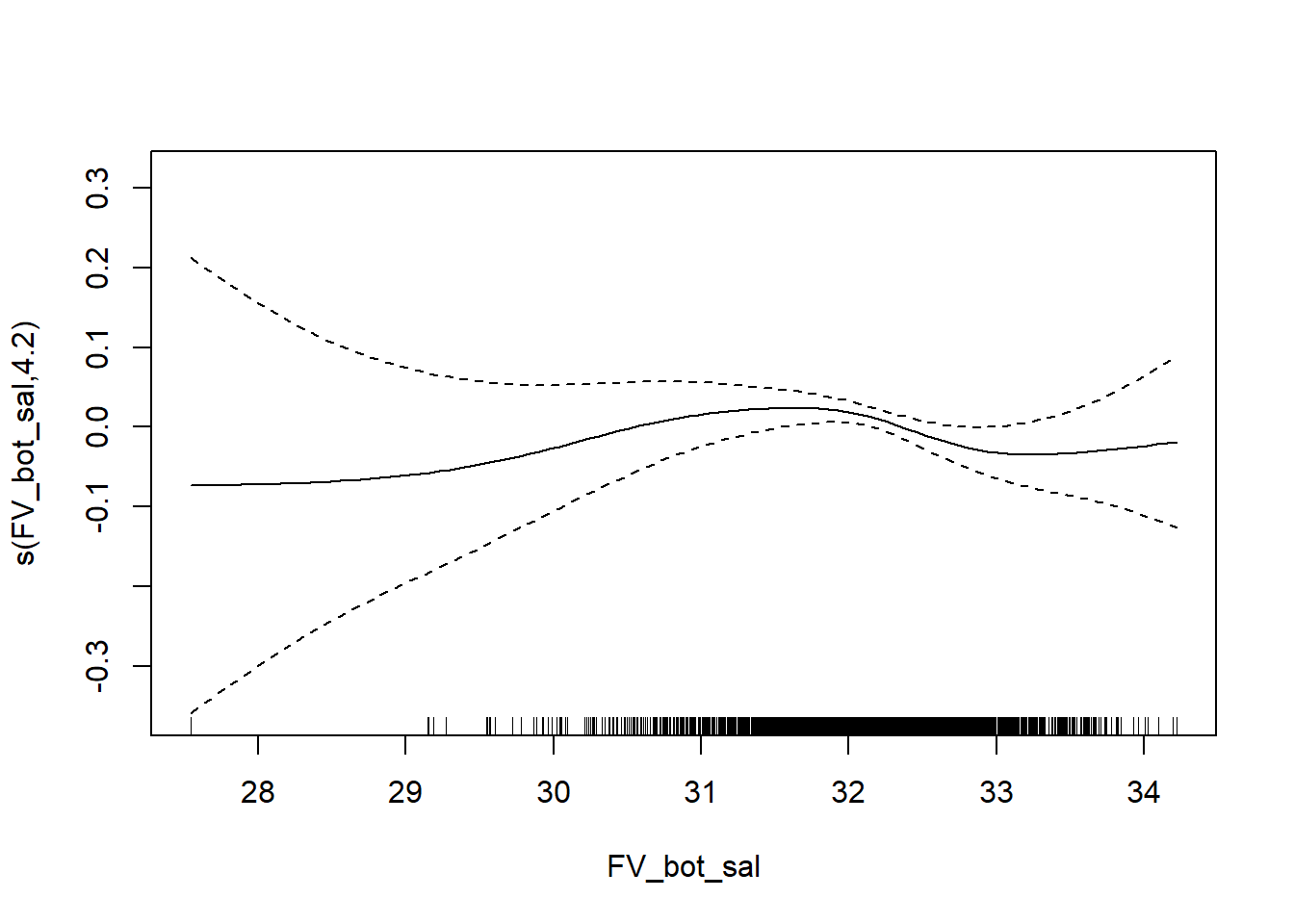
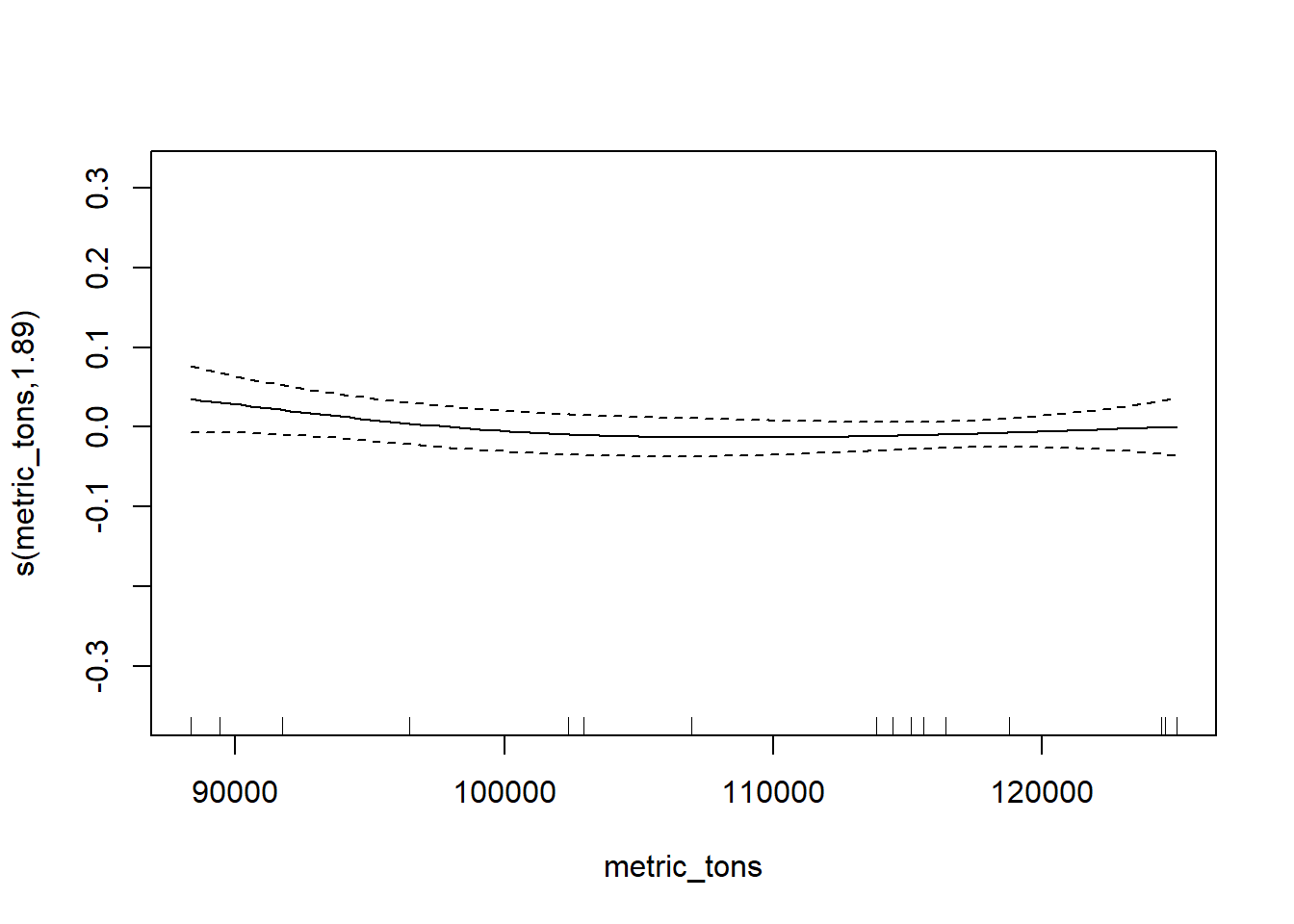
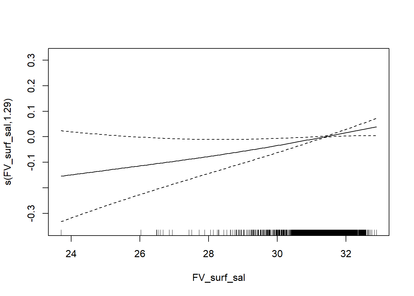
plot(N_Fall_2$gam)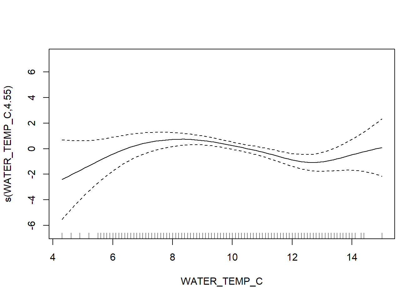
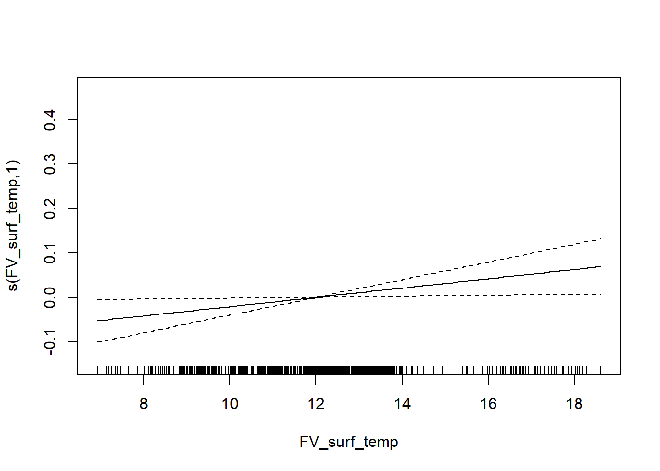
with FVCOM data
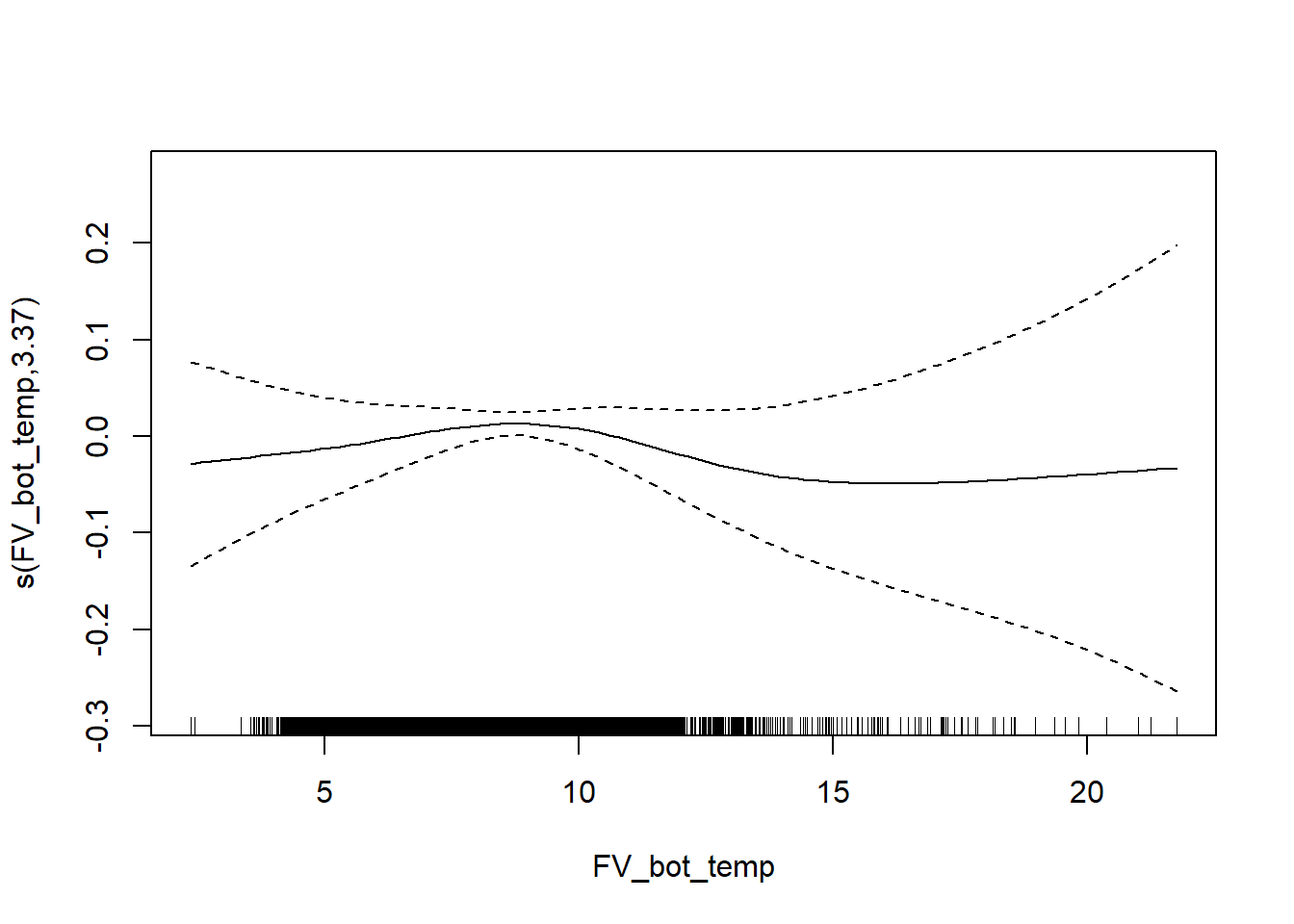
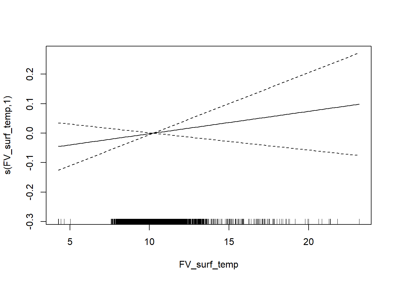
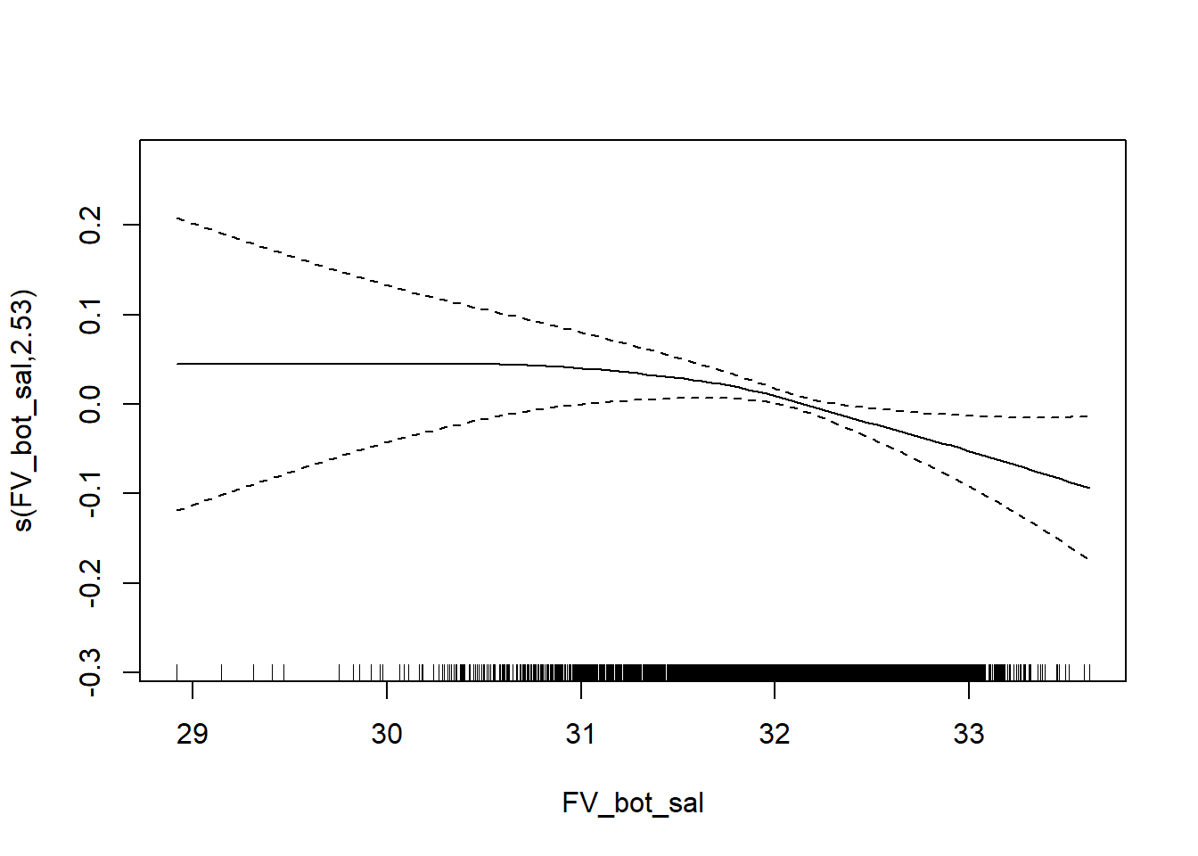
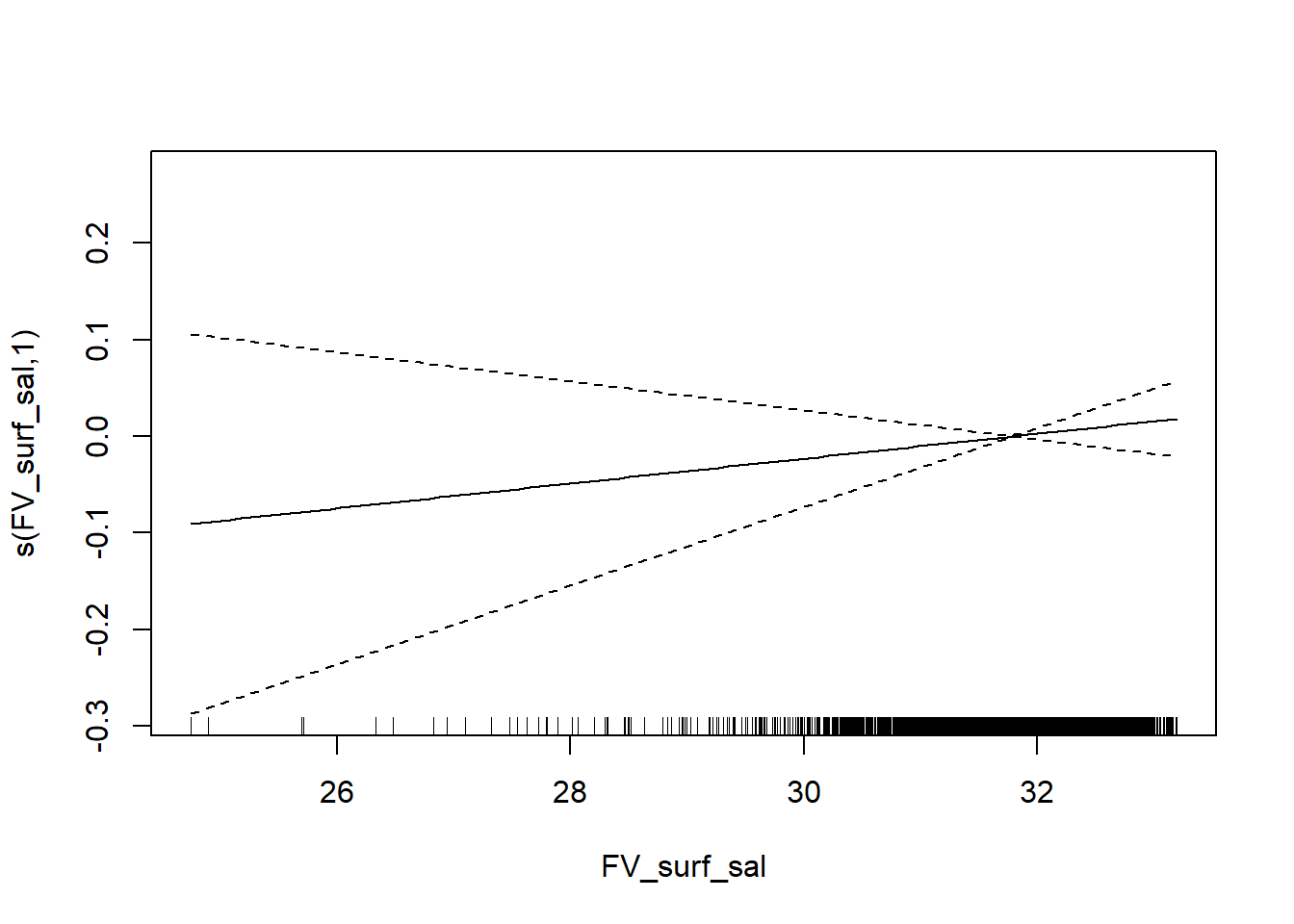
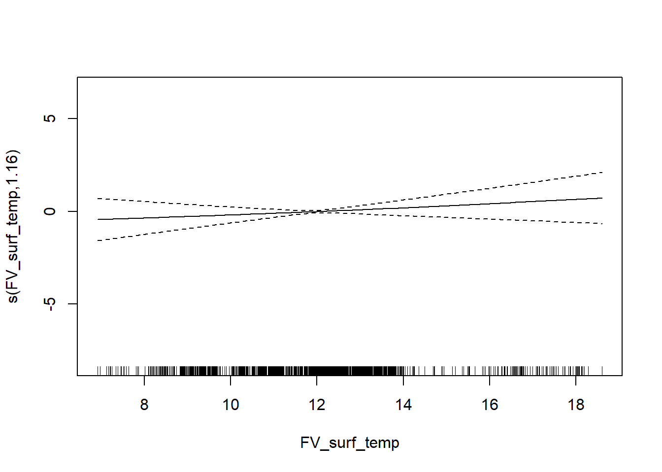
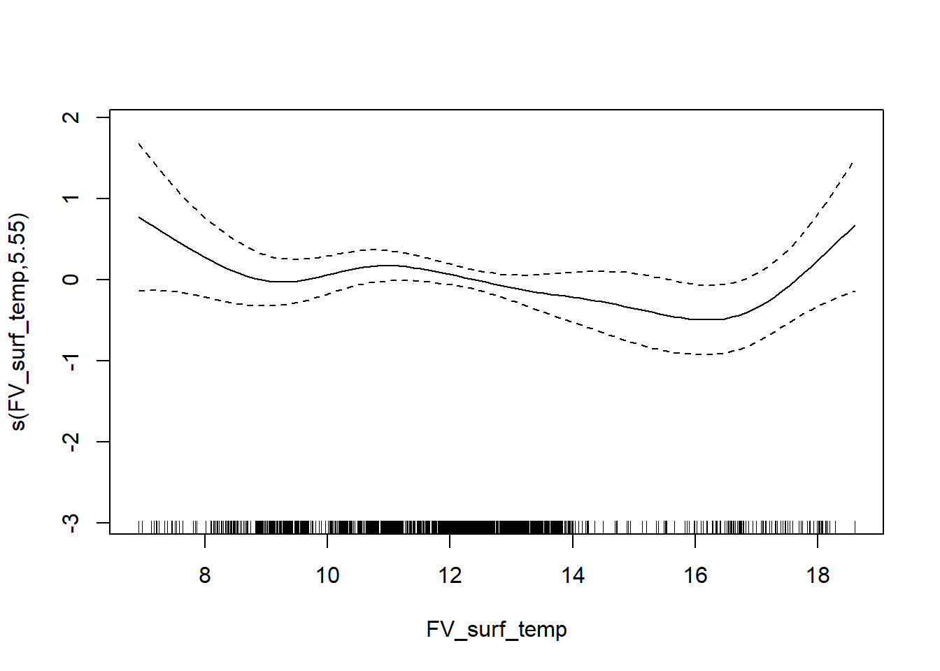
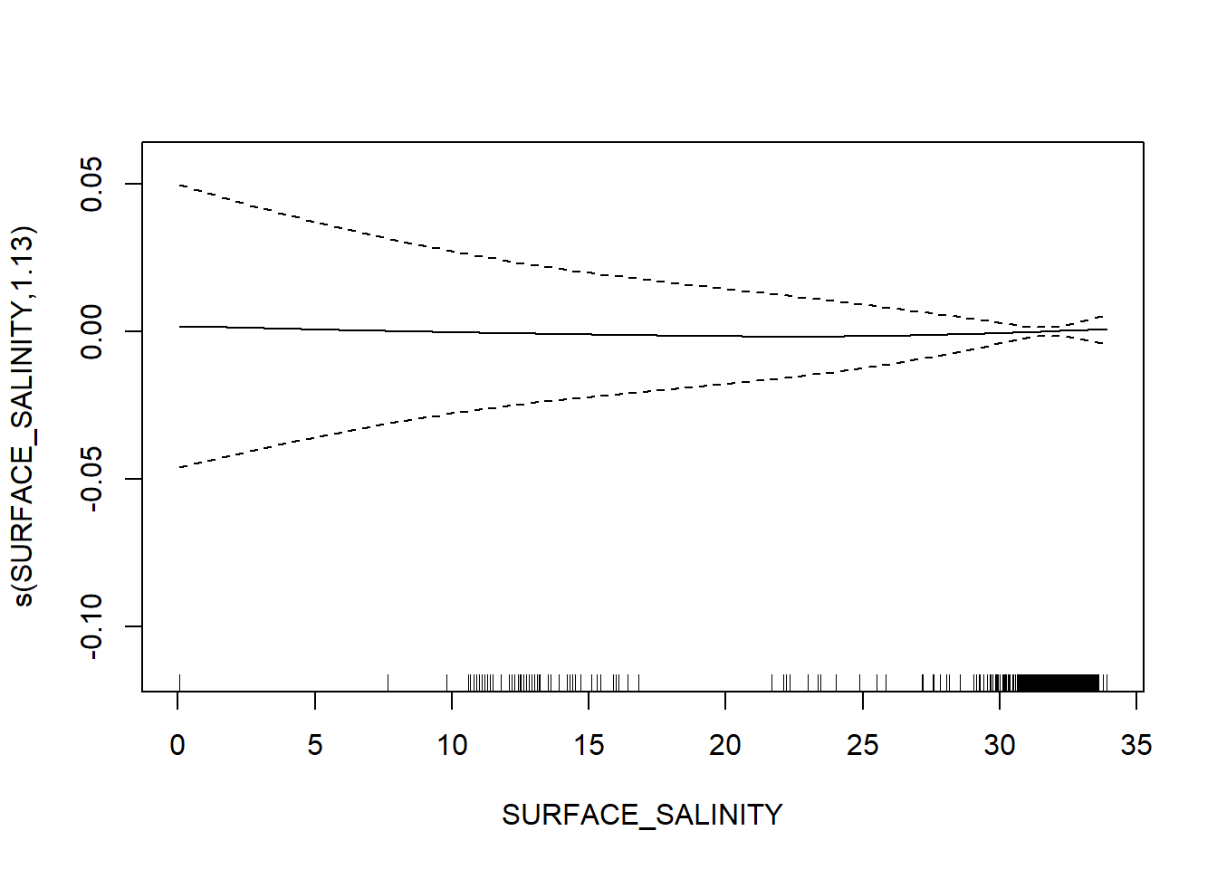
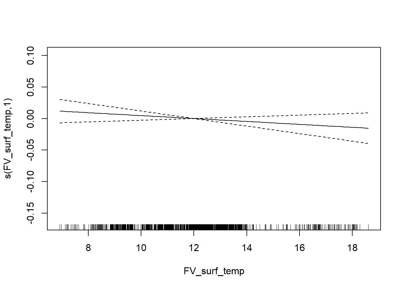
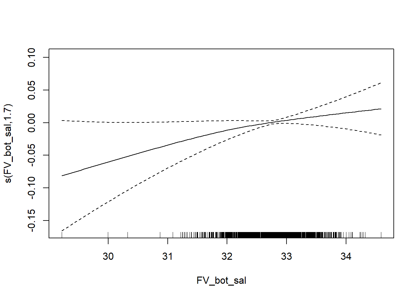
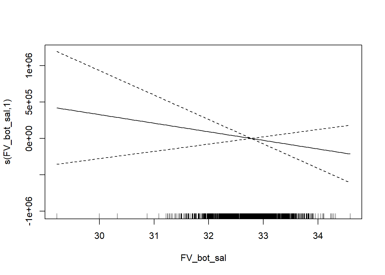
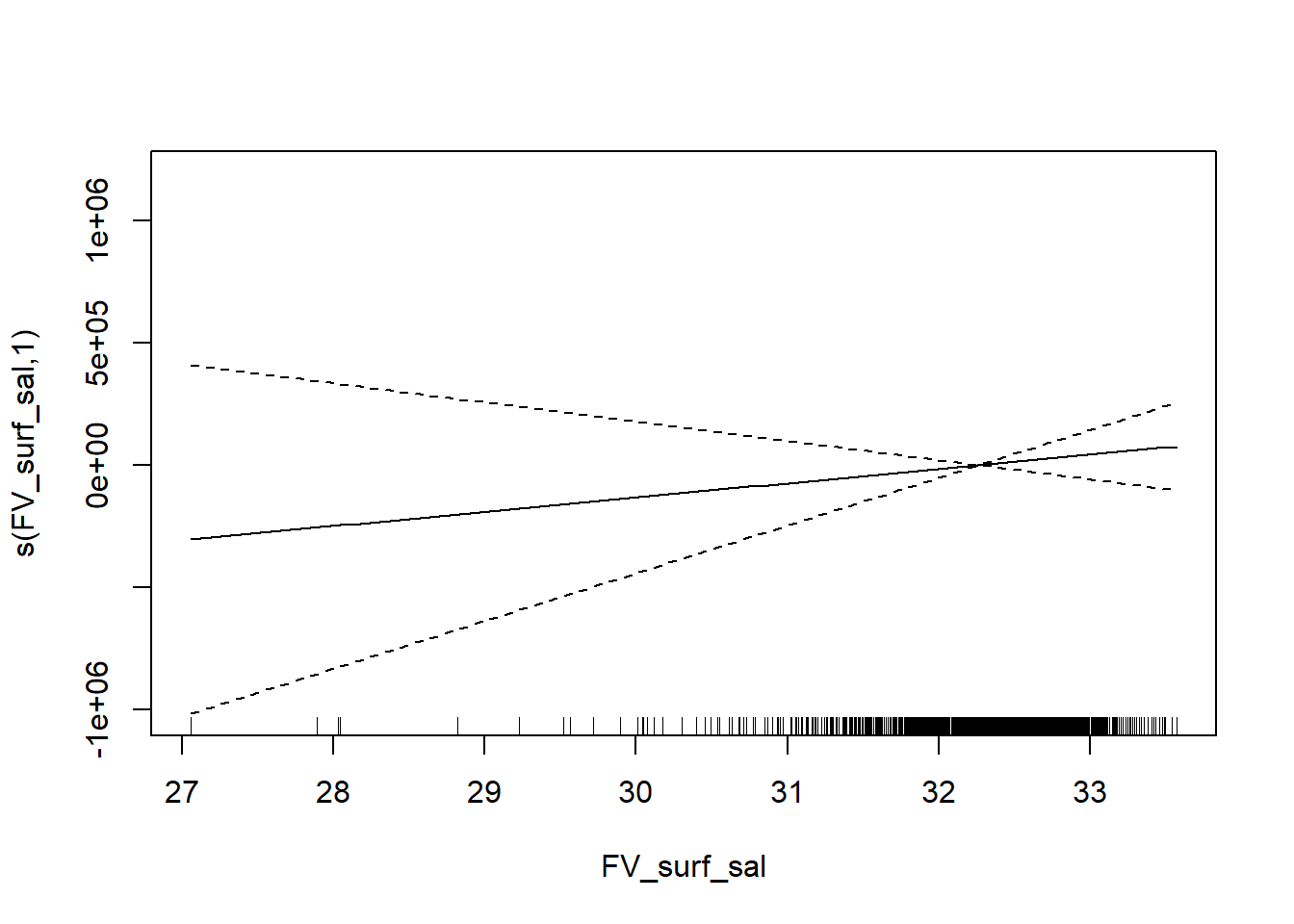
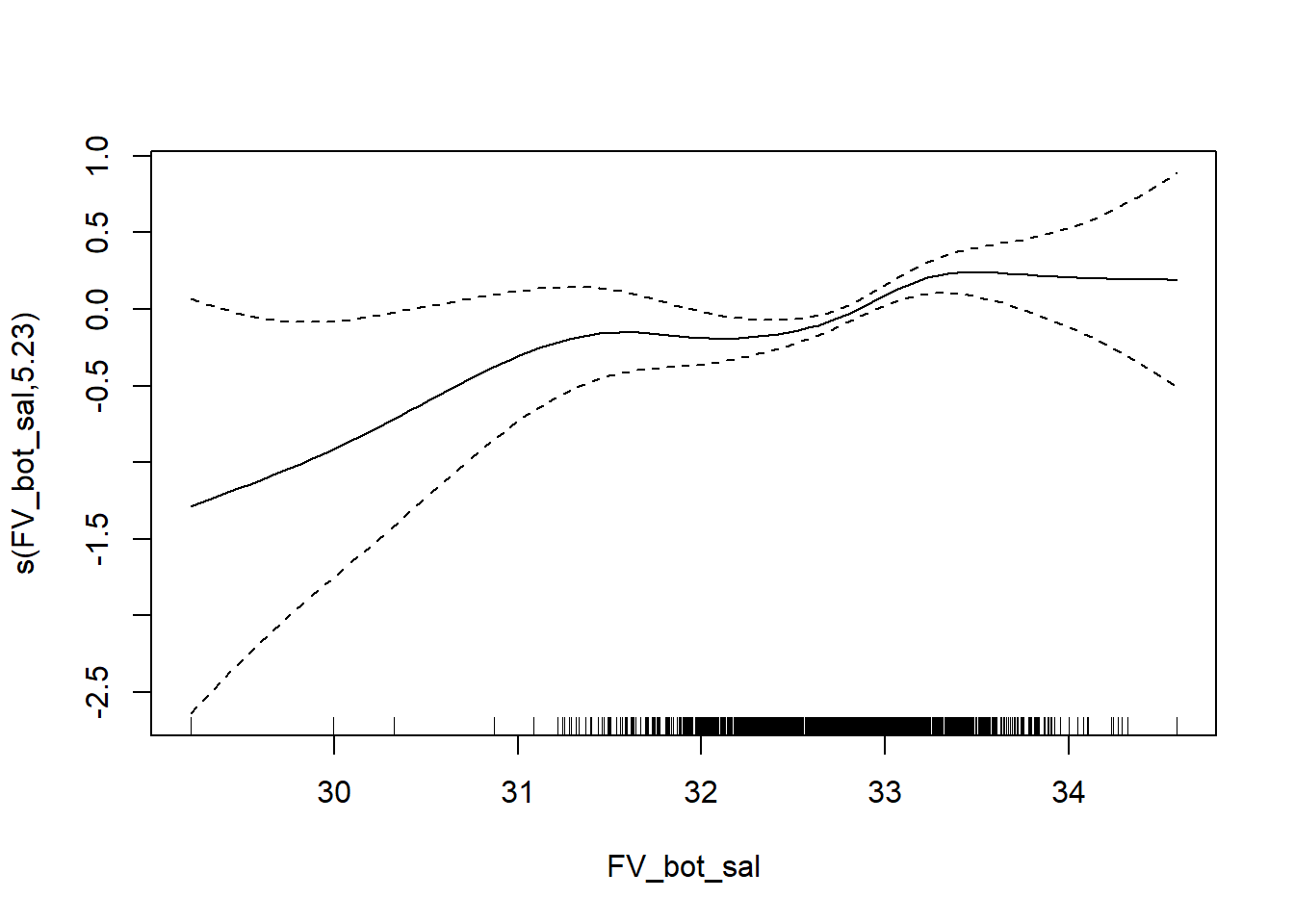
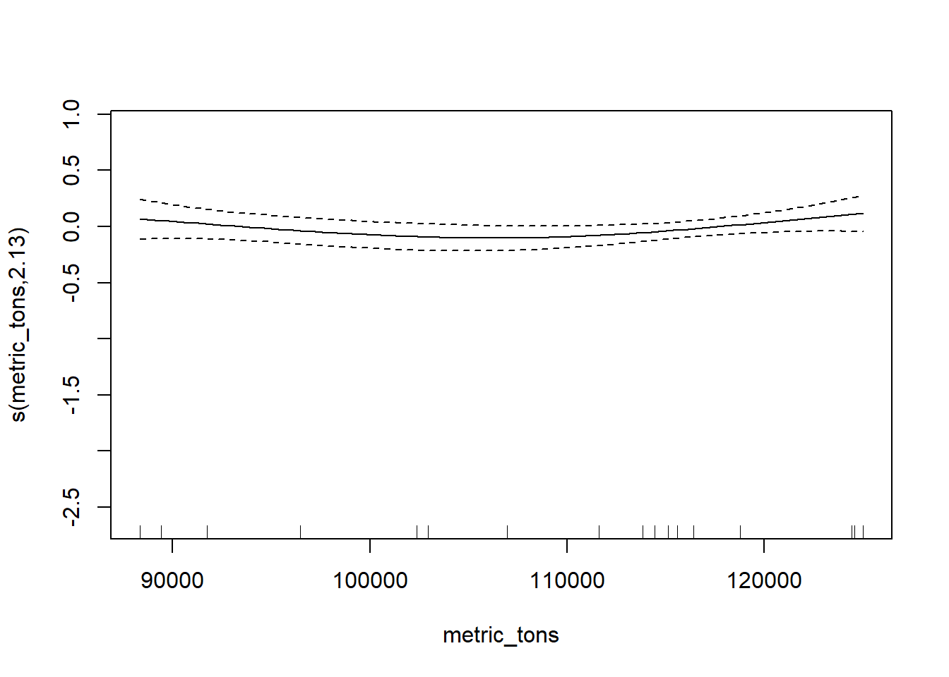
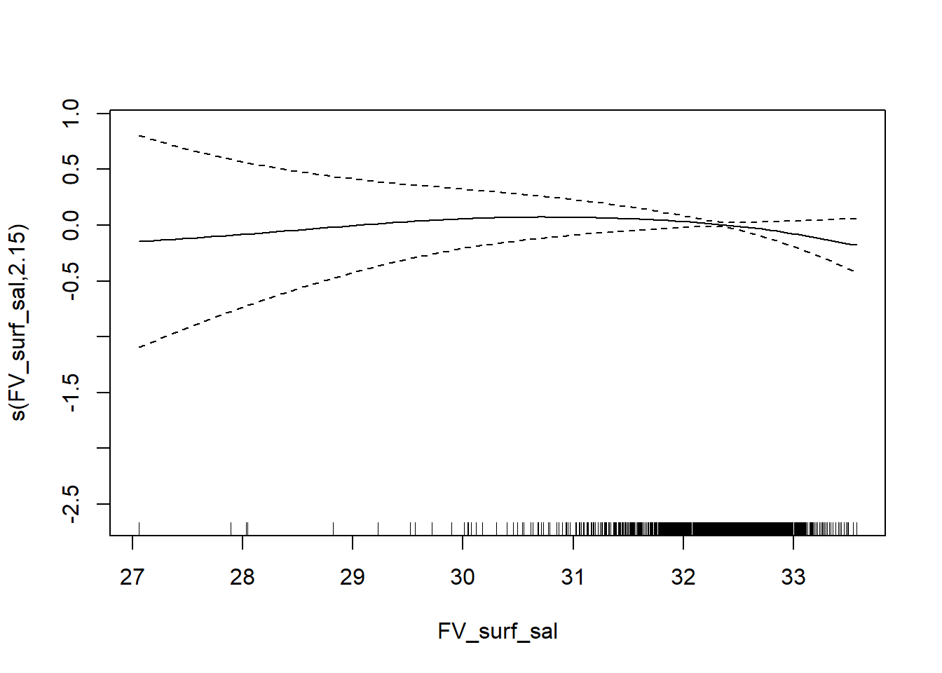
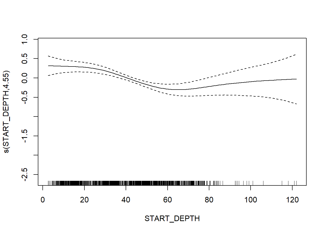
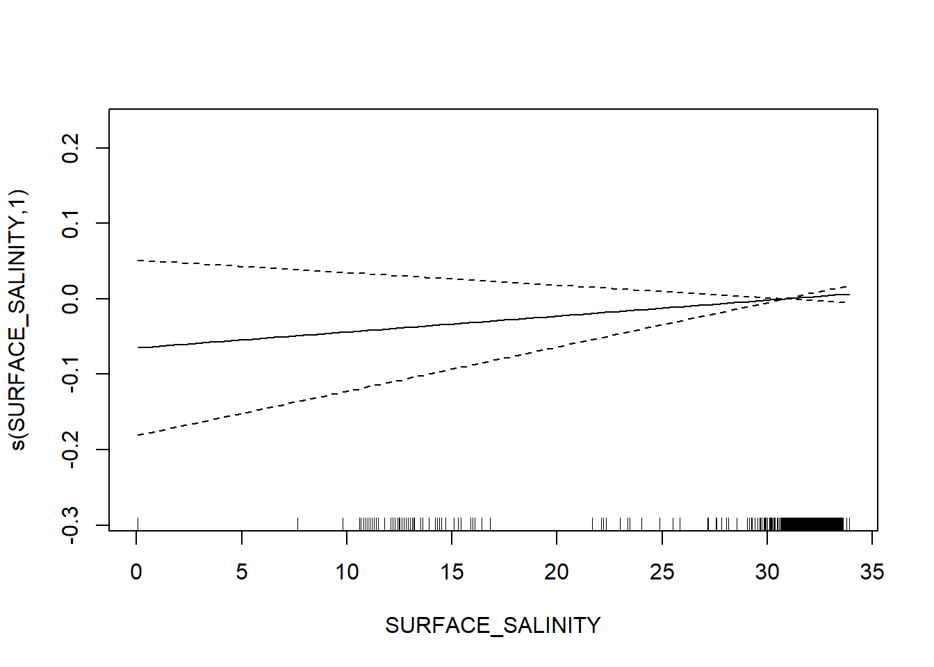
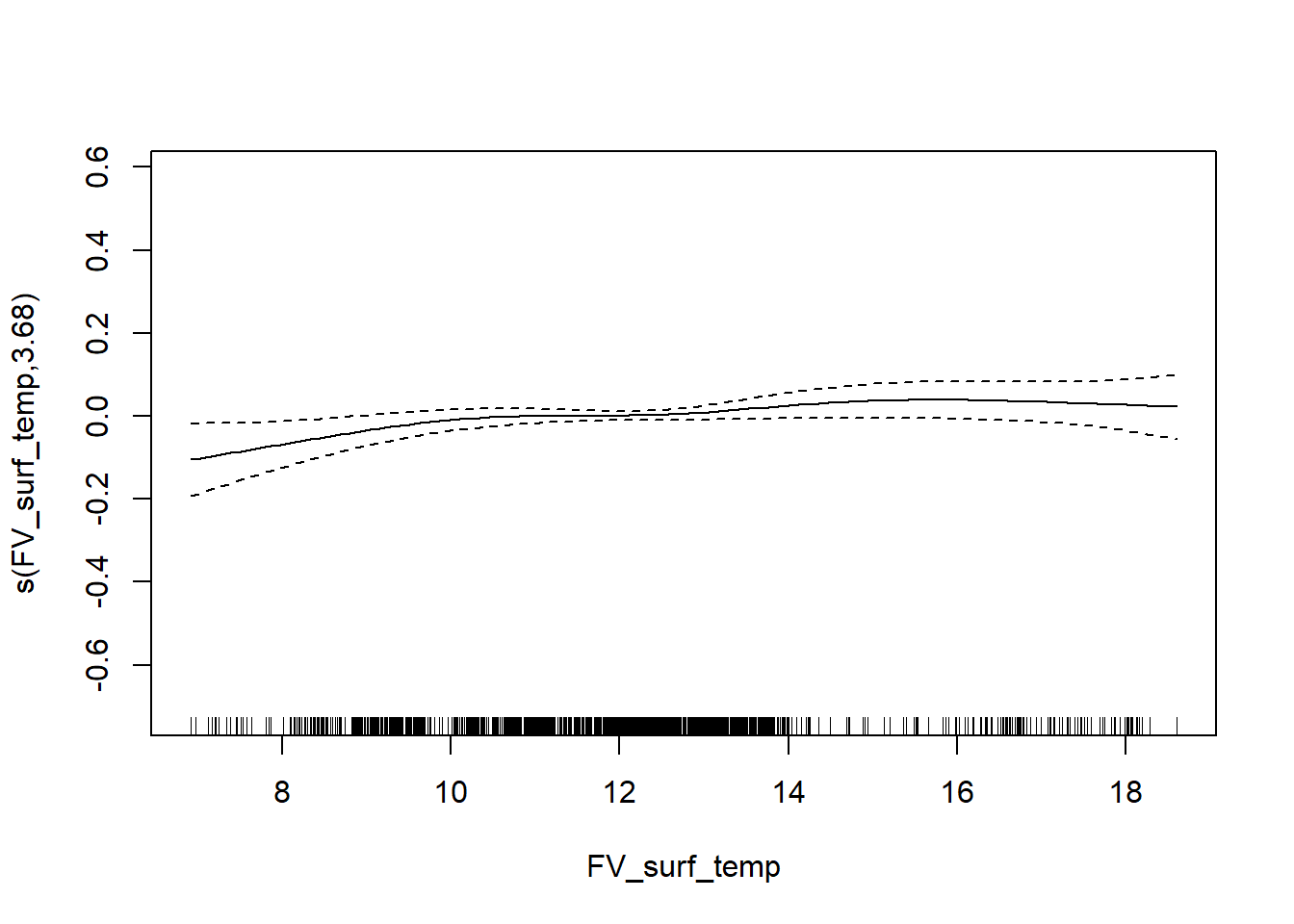
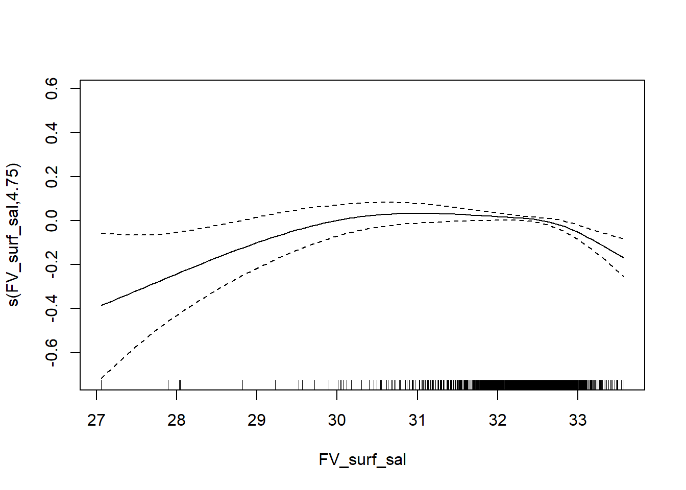
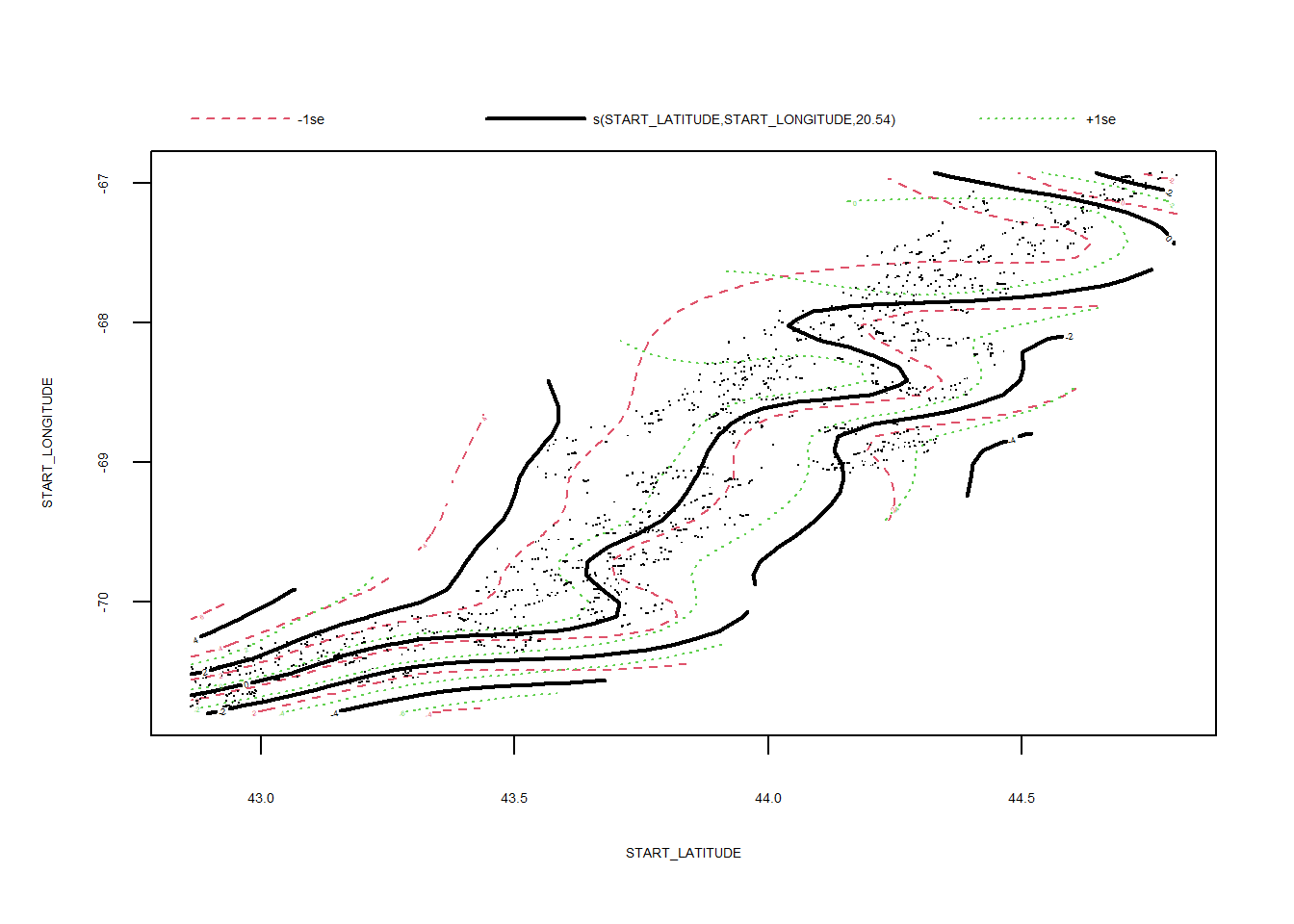
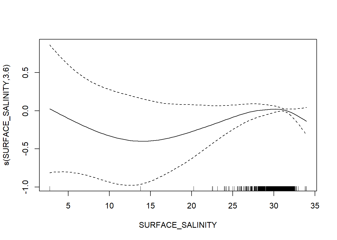
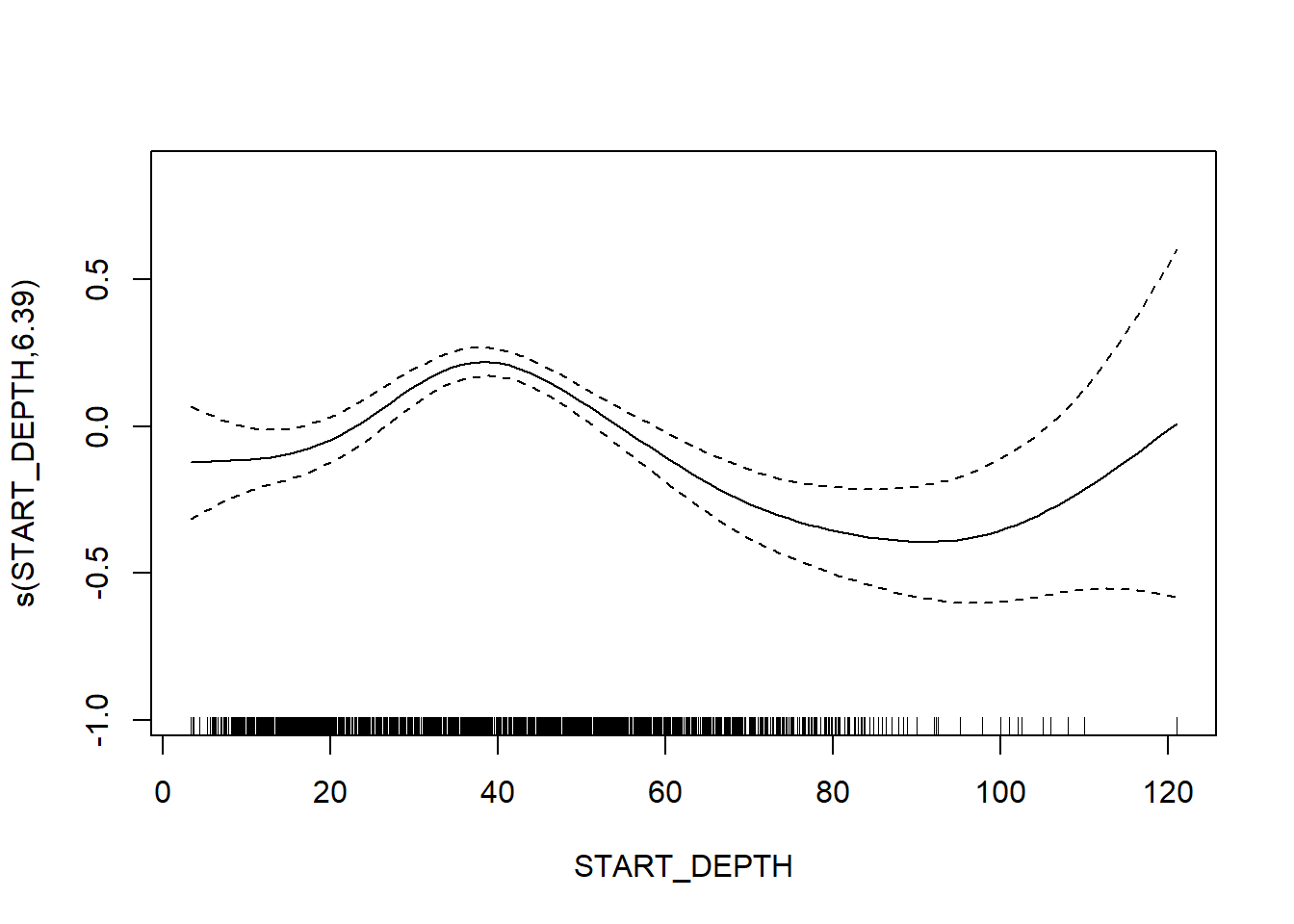
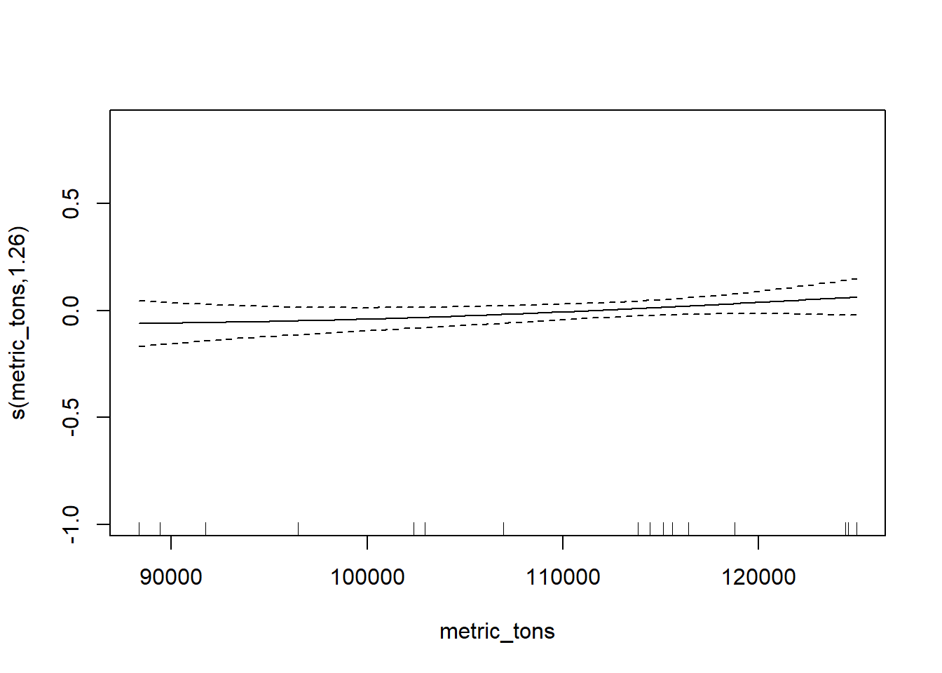
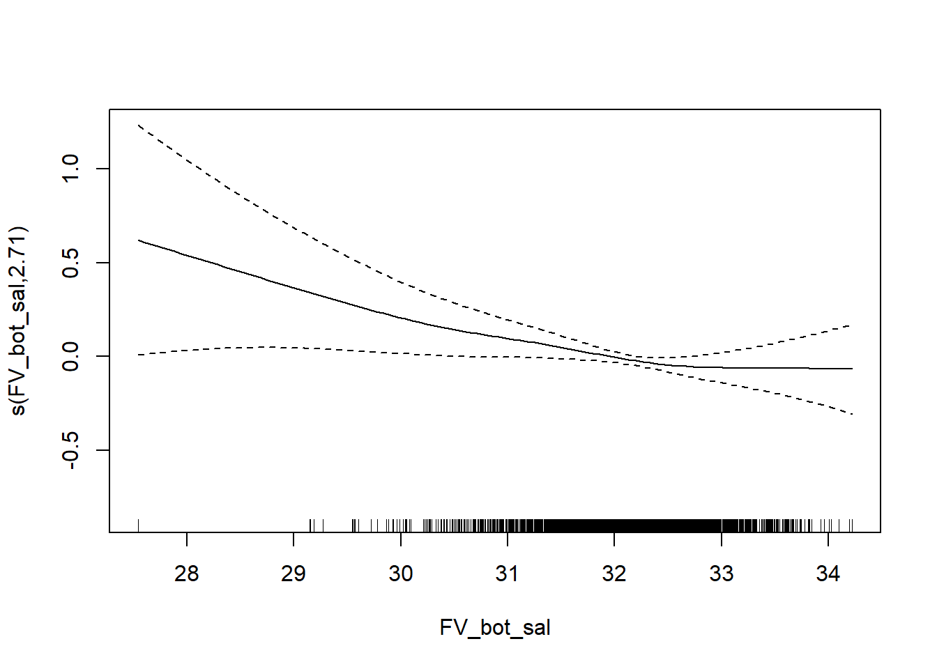
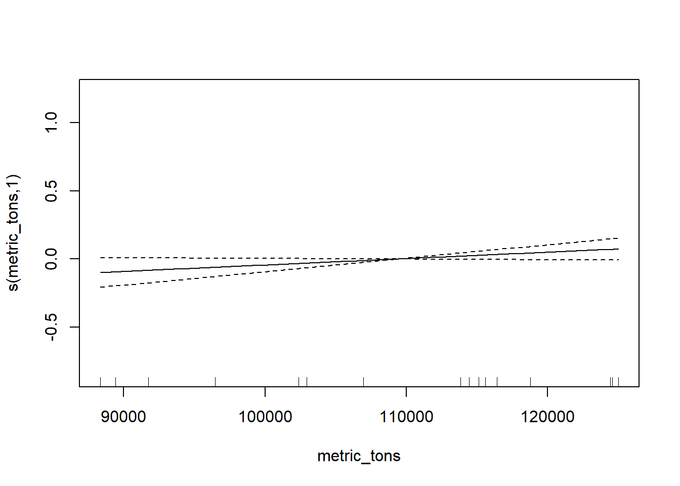
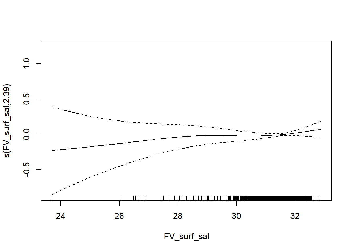
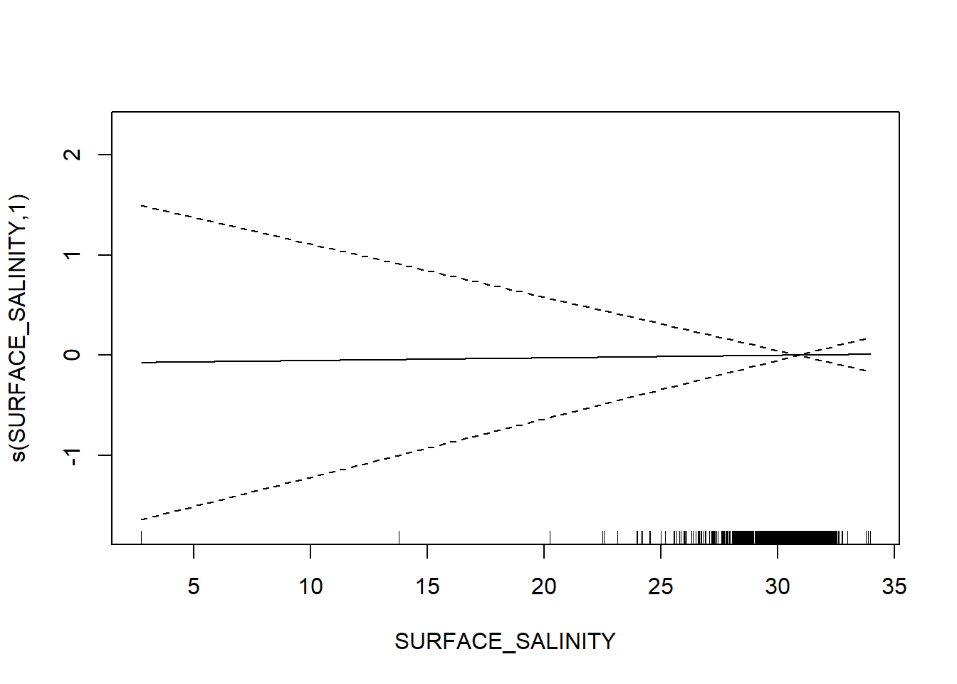
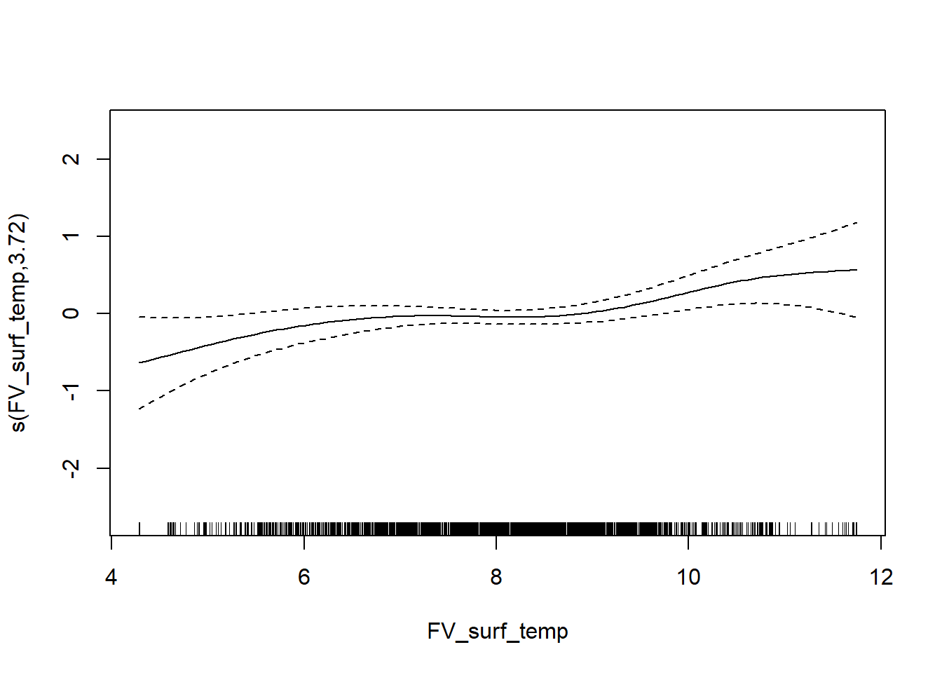
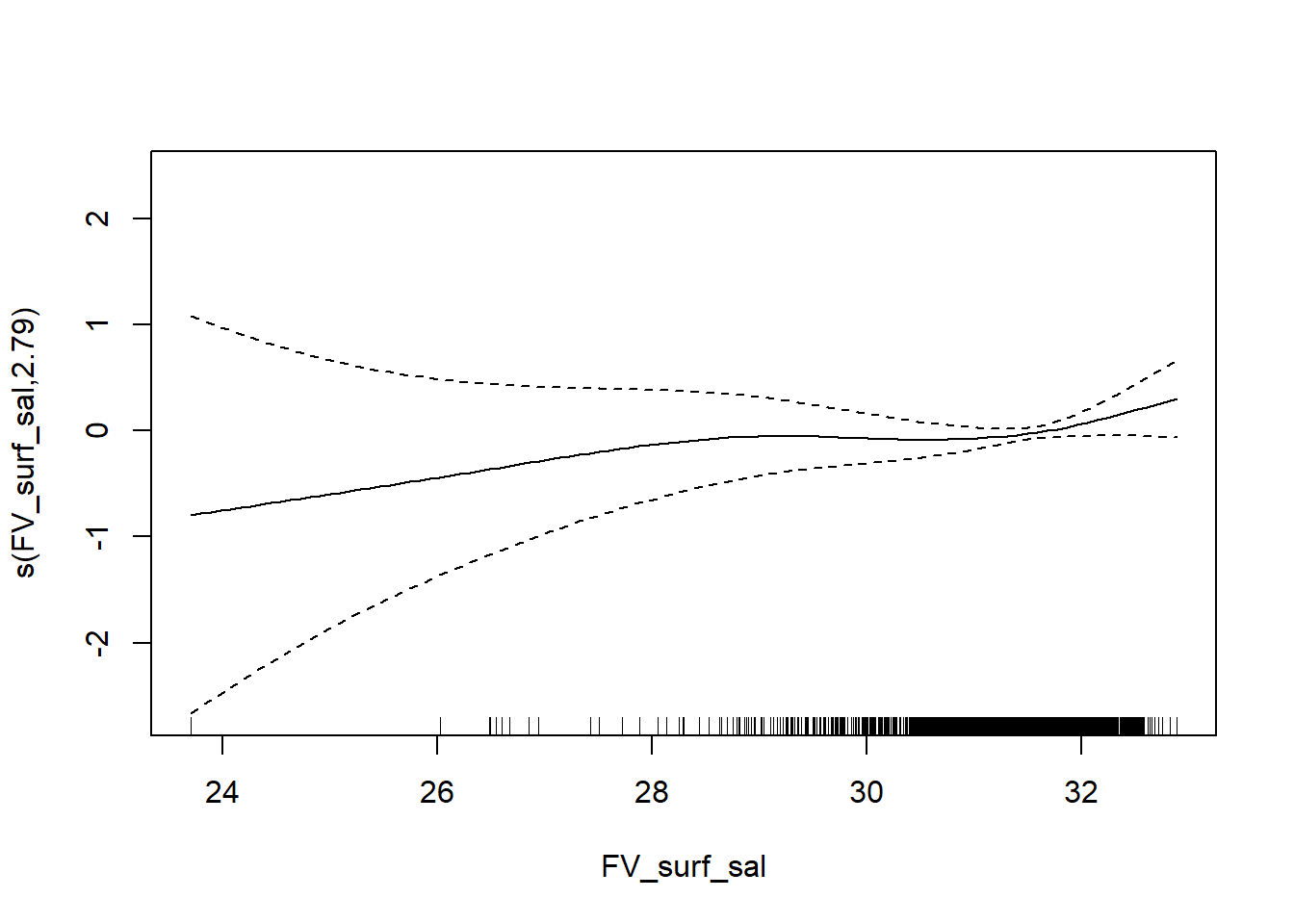
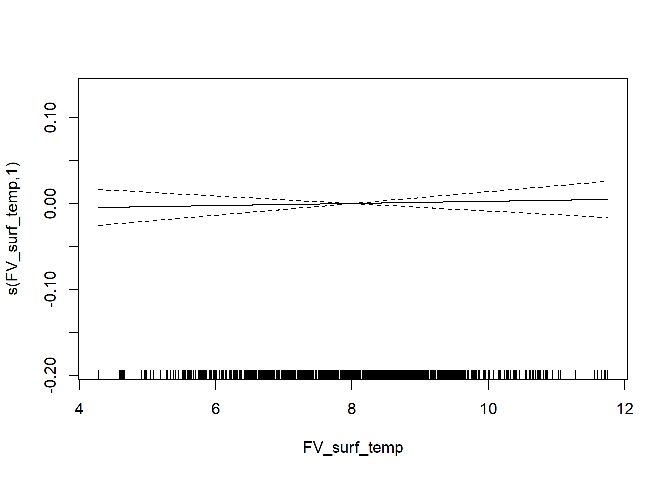
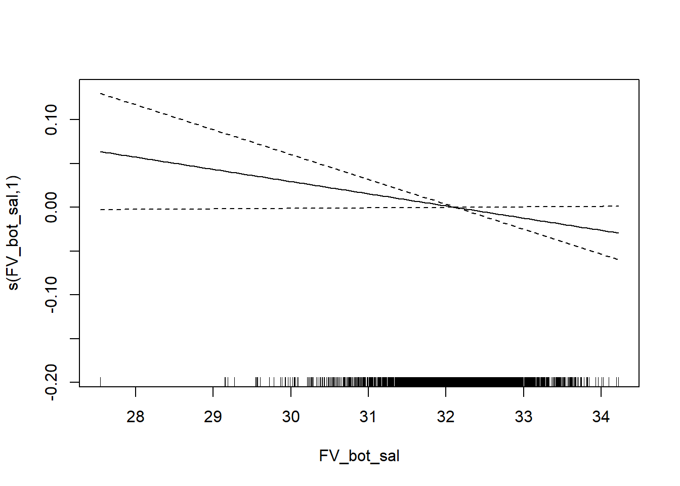
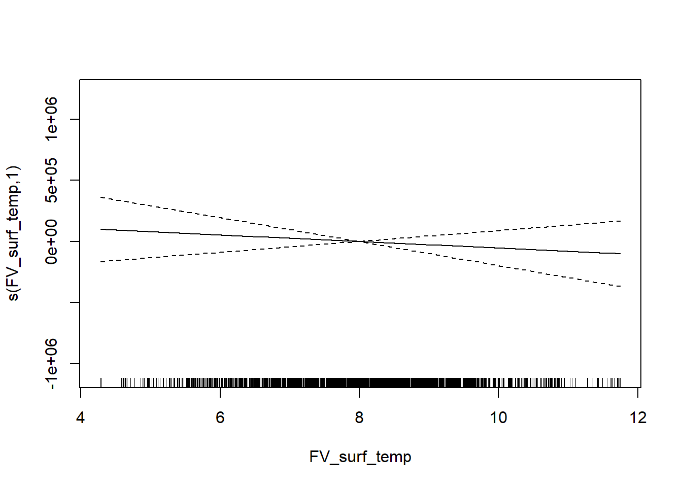
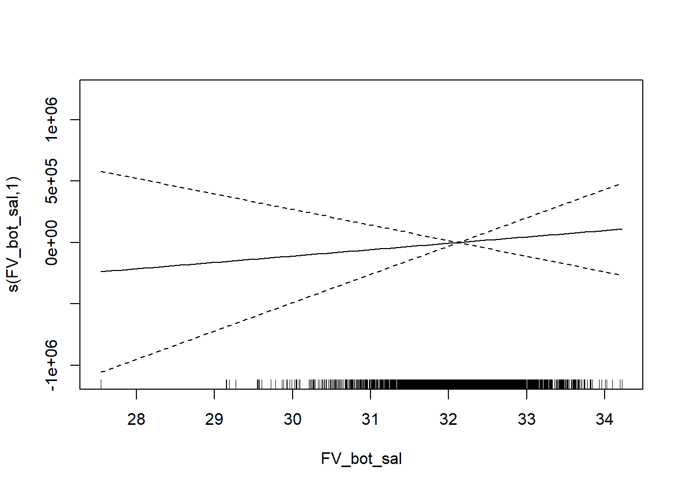
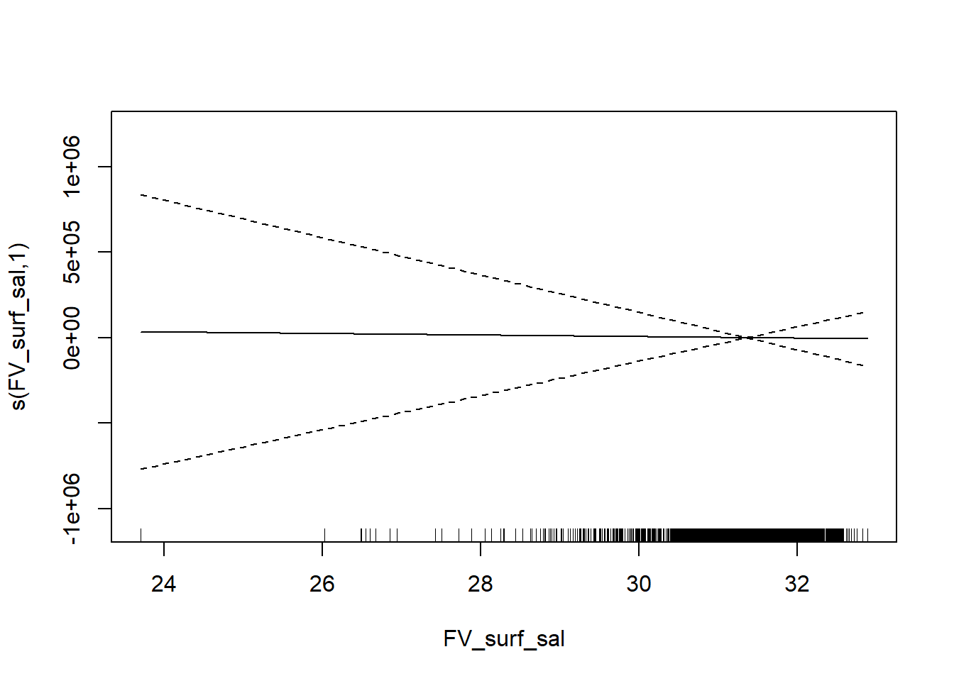
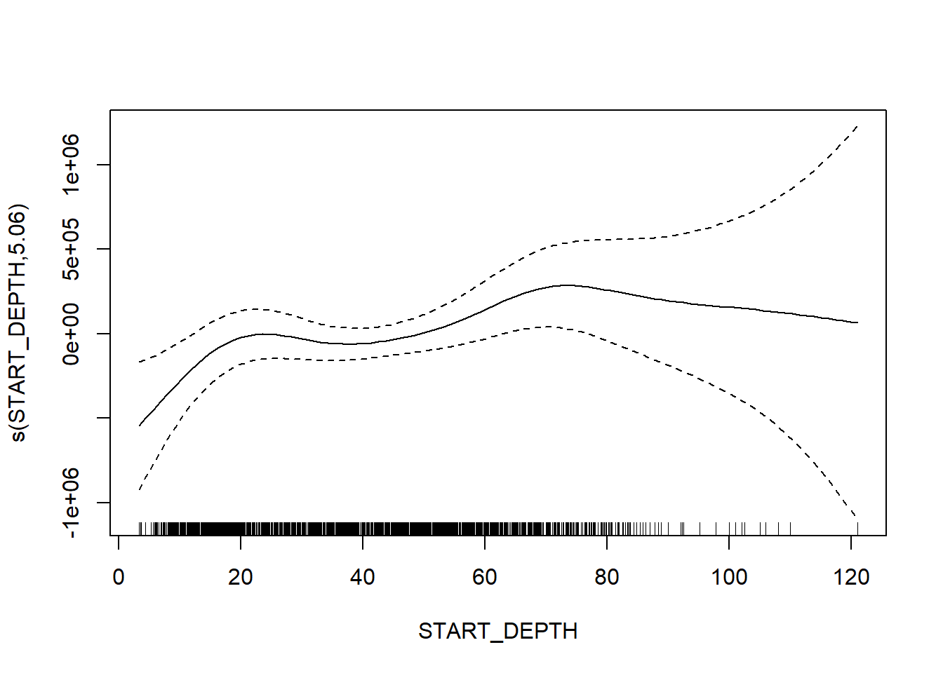
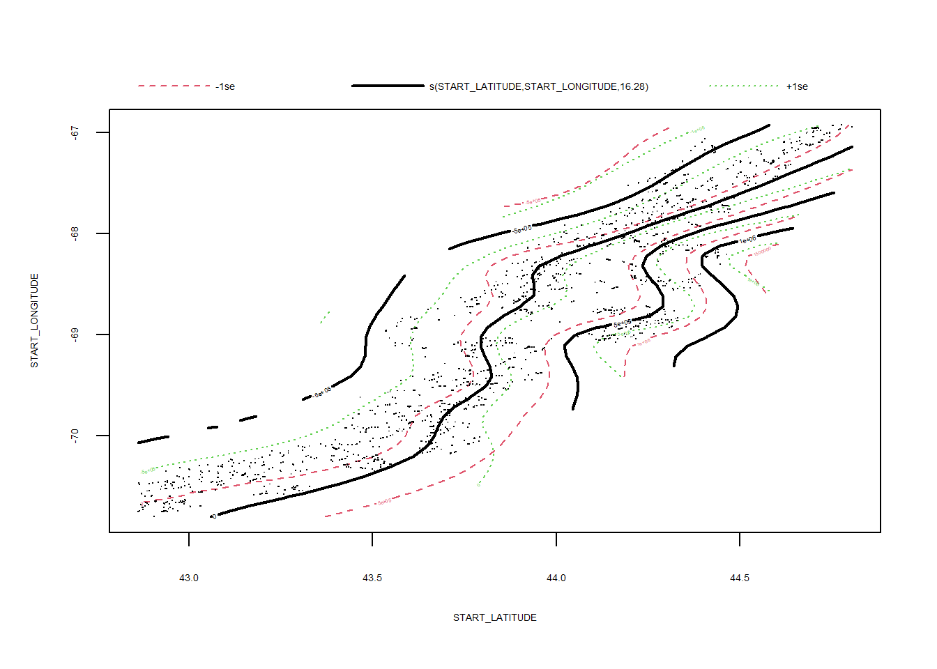
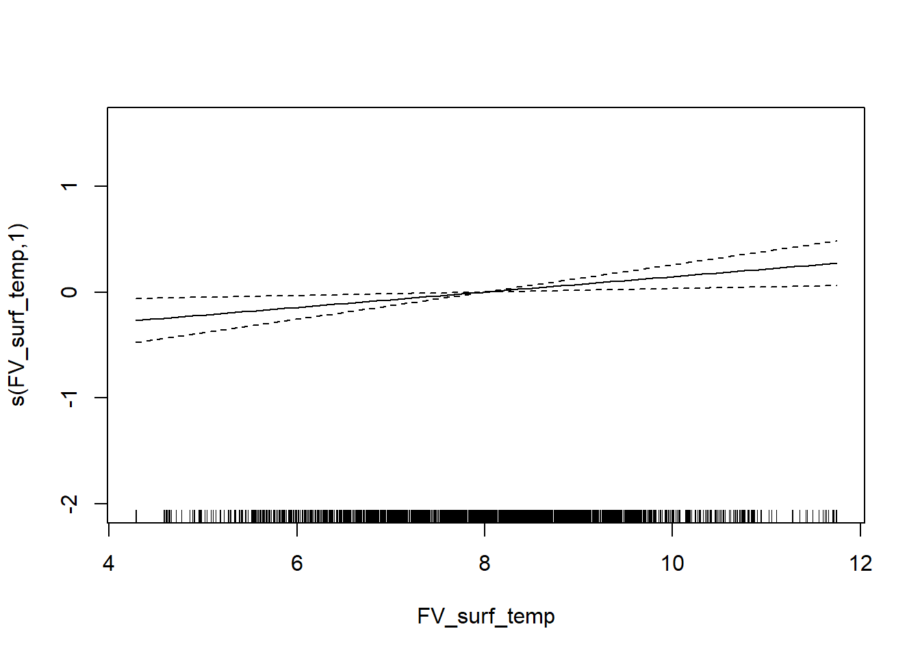
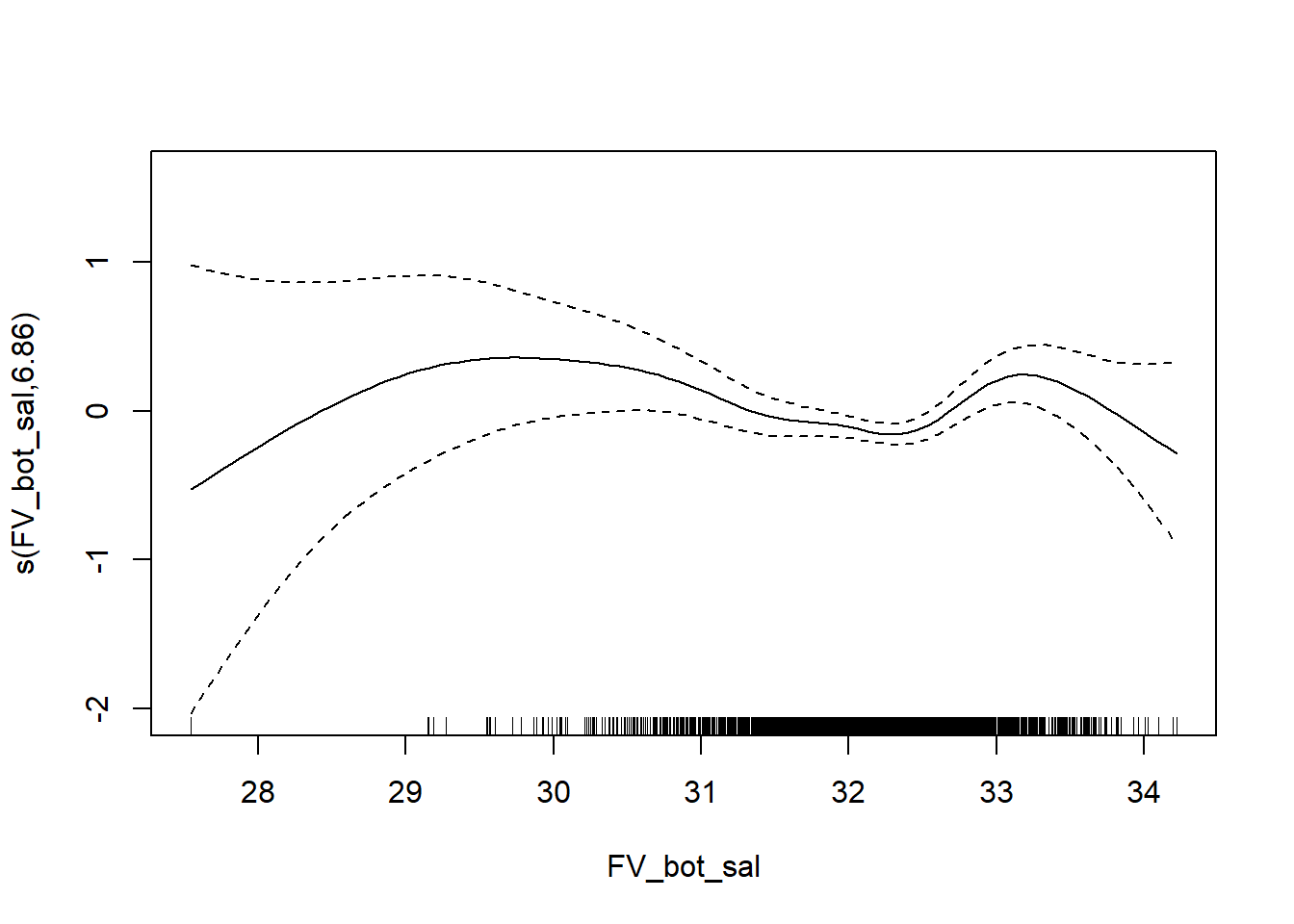
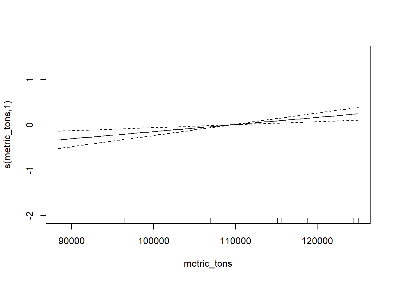
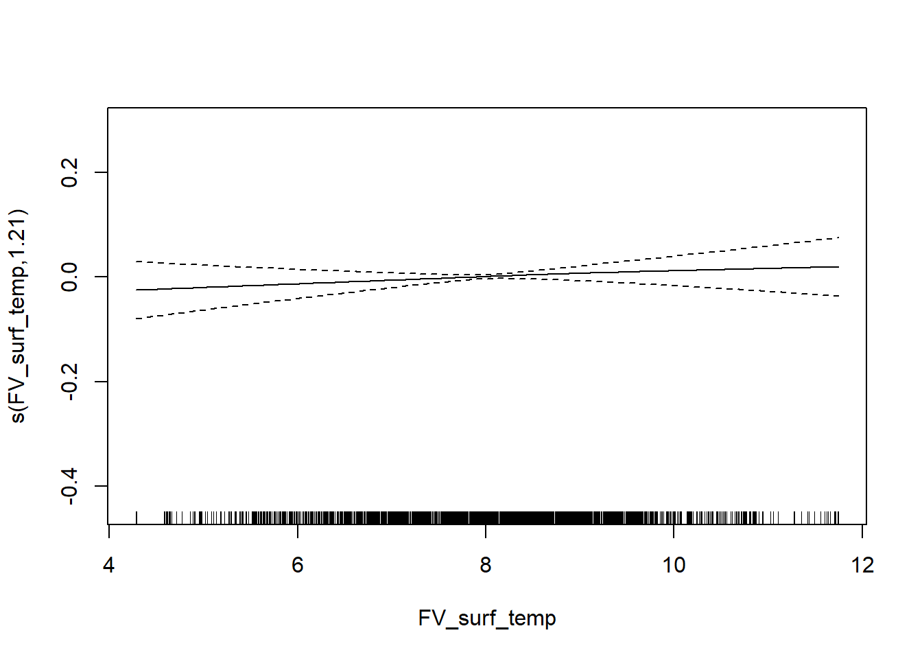
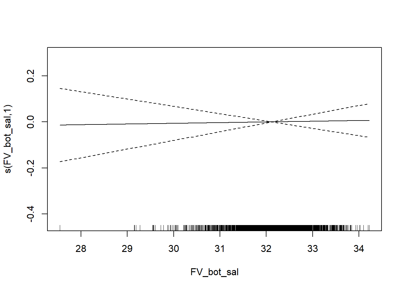
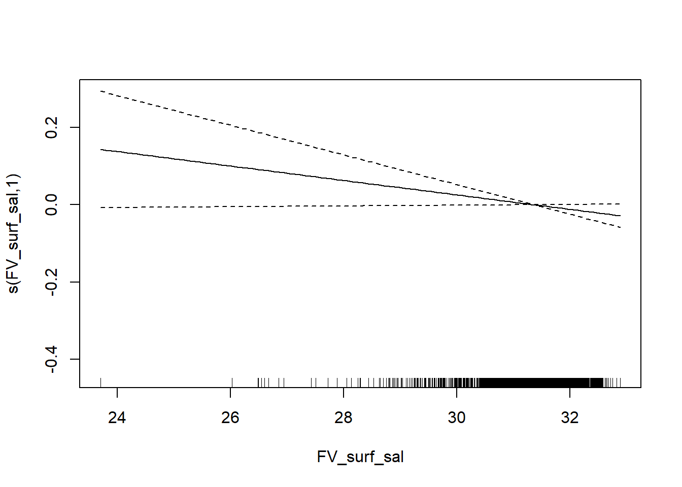
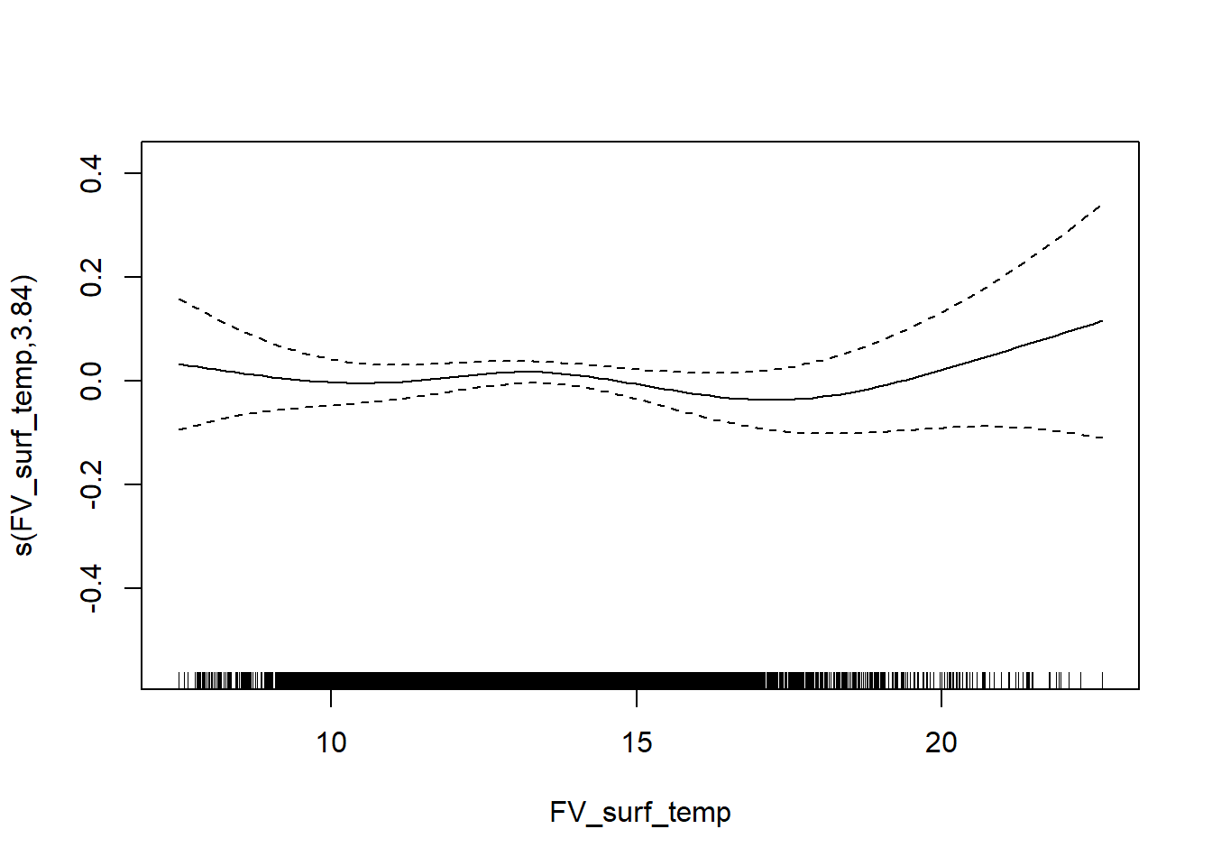
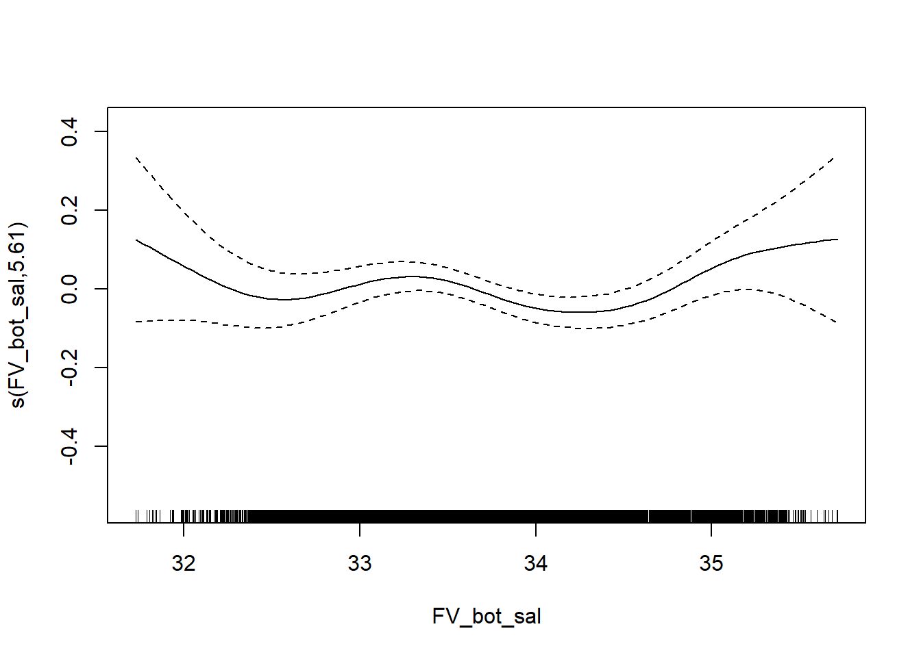
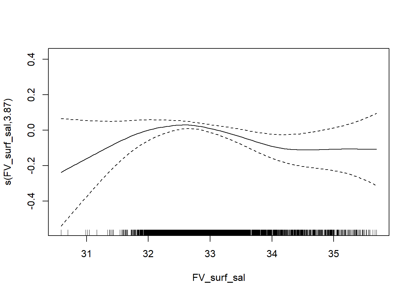
N_Fall_FV <- gamm4(N_species ~ s(FV_bot_temp) + s(FV_surf_temp) + s(FV_bot_sal) +  s(metric_tons) + s(FV_surf_sal) +  s(START_DEPTH) + s(START_LATITUDE, START_LONGITUDE), random = ~ (1|YEAR) , data = fall_fvcom)

gam.check(N_Fall_FV$gam)
##
## 'gamm' based fit - care required with interpretation.
## Checks based on working residuals may be misleading.
## Basis dimension (k) checking results. Low p-value (k-index<1) may
## indicate that k is too low, especially if edf is close to k'.
##
## k' edf k-index p-value
## s(FV_bot_temp) 9.00 4.29 0.99 0.295
## s(FV_surf_temp) 9.00 1.16 1.00 0.435
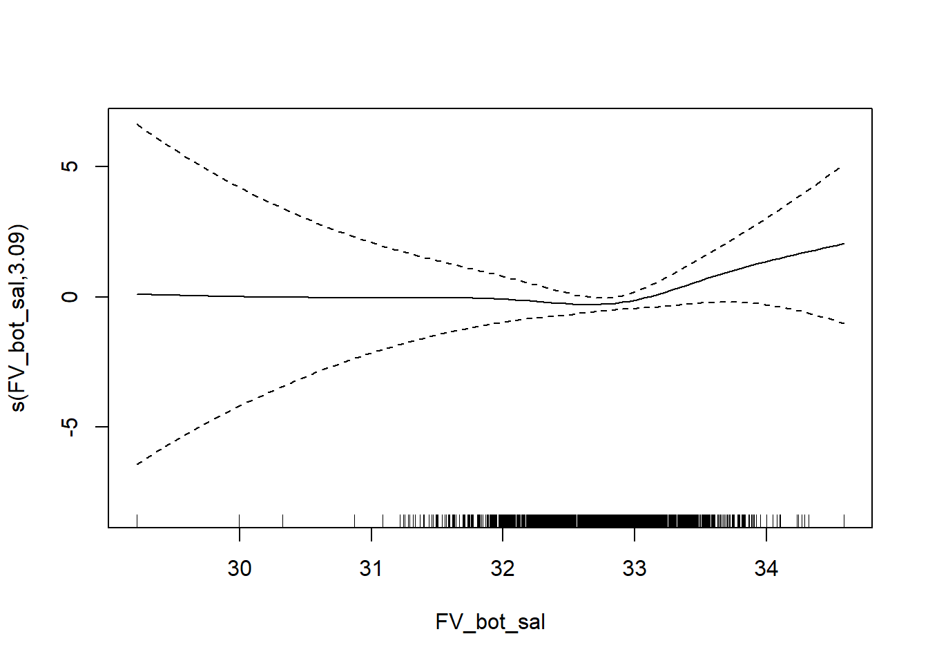
## s(FV_bot_sal) 9.00 3.09 0.95 0.025 *
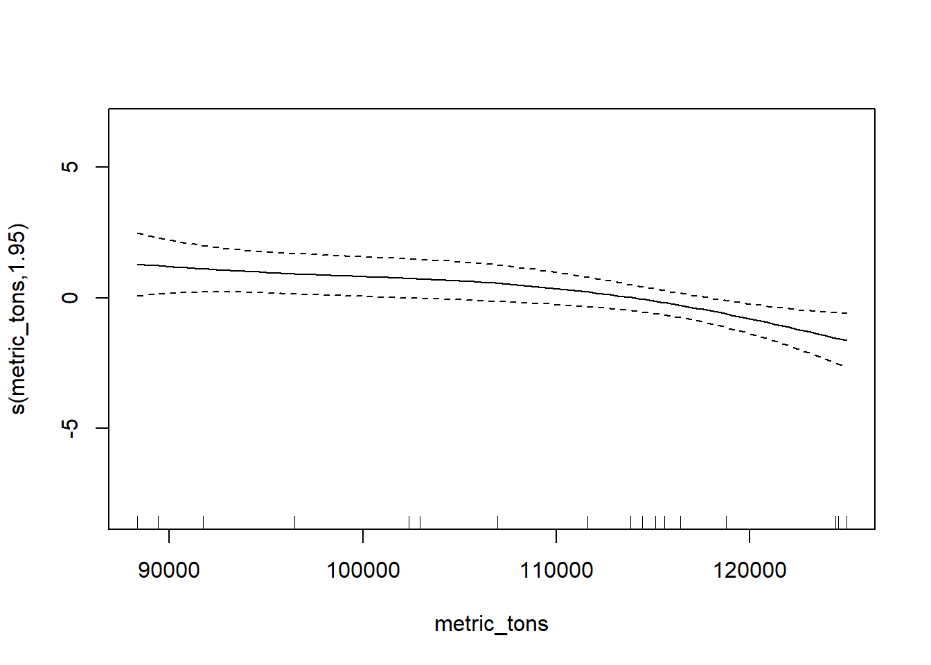
## s(metric_tons) 9.00 1.95 0.79 <2e-16 ***
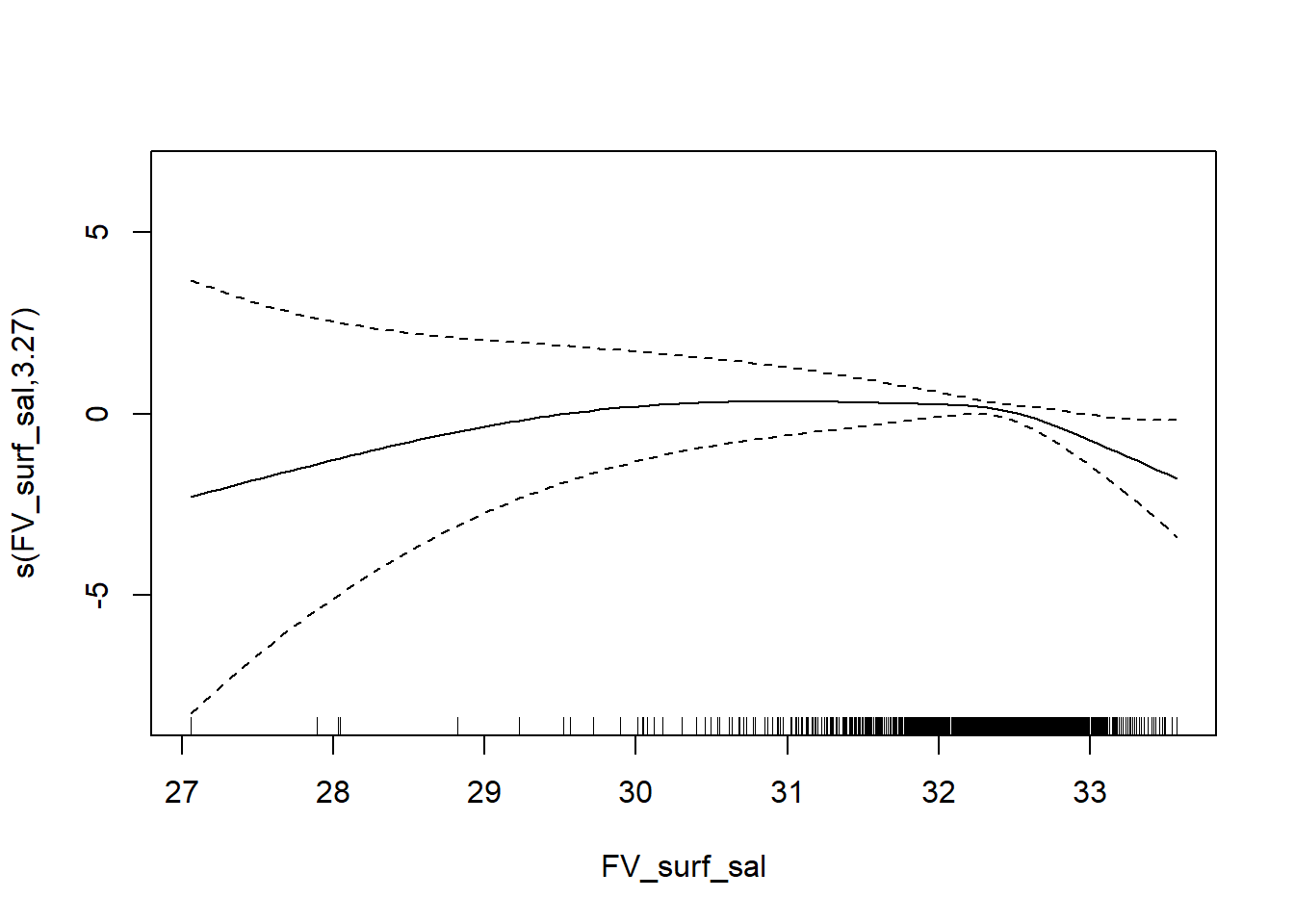
## s(FV_surf_sal) 9.00 3.27 1.00 0.385
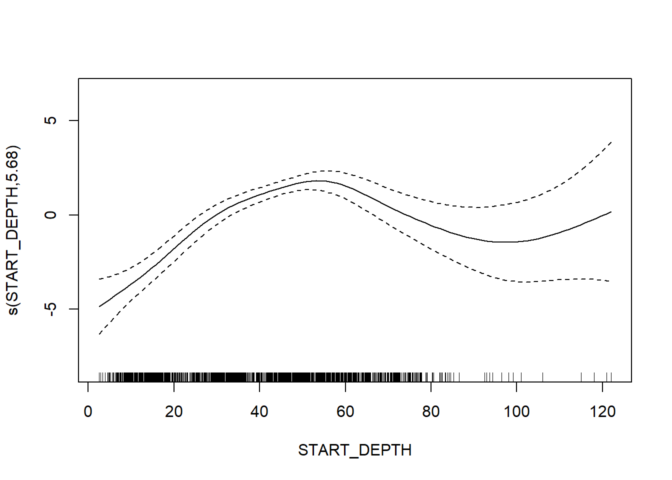
## s(START_DEPTH) 9.00 5.68 0.97 0.095 .
## s(START_LATITUDE,START_LONGITUDE) 29.00 16.69 0.94 <2e-16 ***
## ---
## Signif. codes: 0 '***' 0.001 '**' 0.01 '*' 0.05 '.' 0.1 ' ' 1summary(N_Fall_FV$gam)##
## Family: gaussian
## Link function: identity
##
## Formula:
## N_species ~ s(FV_bot_temp) + s(FV_surf_temp) + s(FV_bot_sal) +
## s(metric_tons) + s(FV_surf_sal) + s(START_DEPTH) + s(START_LATITUDE,
## START_LONGITUDE)
##
## Parametric coefficients:
## Estimate Std. Error t value Pr(>|t|)
## (Intercept) 21.179 0.265 79.92 <2e-16 ***
## ---
## Signif. codes: 0 '***' 0.001 '**' 0.01 '*' 0.05 '.' 0.1 ' ' 1
##
## Approximate significance of smooth terms:
## edf Ref.df F p-value
## s(FV_bot_temp) 4.289 4.289 10.188 < 2e-16 ***
## s(FV_surf_temp) 1.156 1.156 1.028 0.3794
## s(FV_bot_sal) 3.091 3.091 1.704 0.1727
## s(metric_tons) 1.953 1.953 5.256 0.0045 **
## s(FV_surf_sal) 3.267 3.267 1.479 0.1683
## s(START_DEPTH) 5.681 5.681 27.290 < 2e-16 ***
## s(START_LATITUDE,START_LONGITUDE) 16.689 16.689 3.379 5.3e-06 ***
## ---
## Signif. codes: 0 '***' 0.001 '**' 0.01 '*' 0.05 '.' 0.1 ' ' 1
##
## R-sq.(adj) = 0.396
## lmer.REML = 7599.1 Scale est. = 11.616 n = 1417#plot(resid(N_Fall_FV$gam))
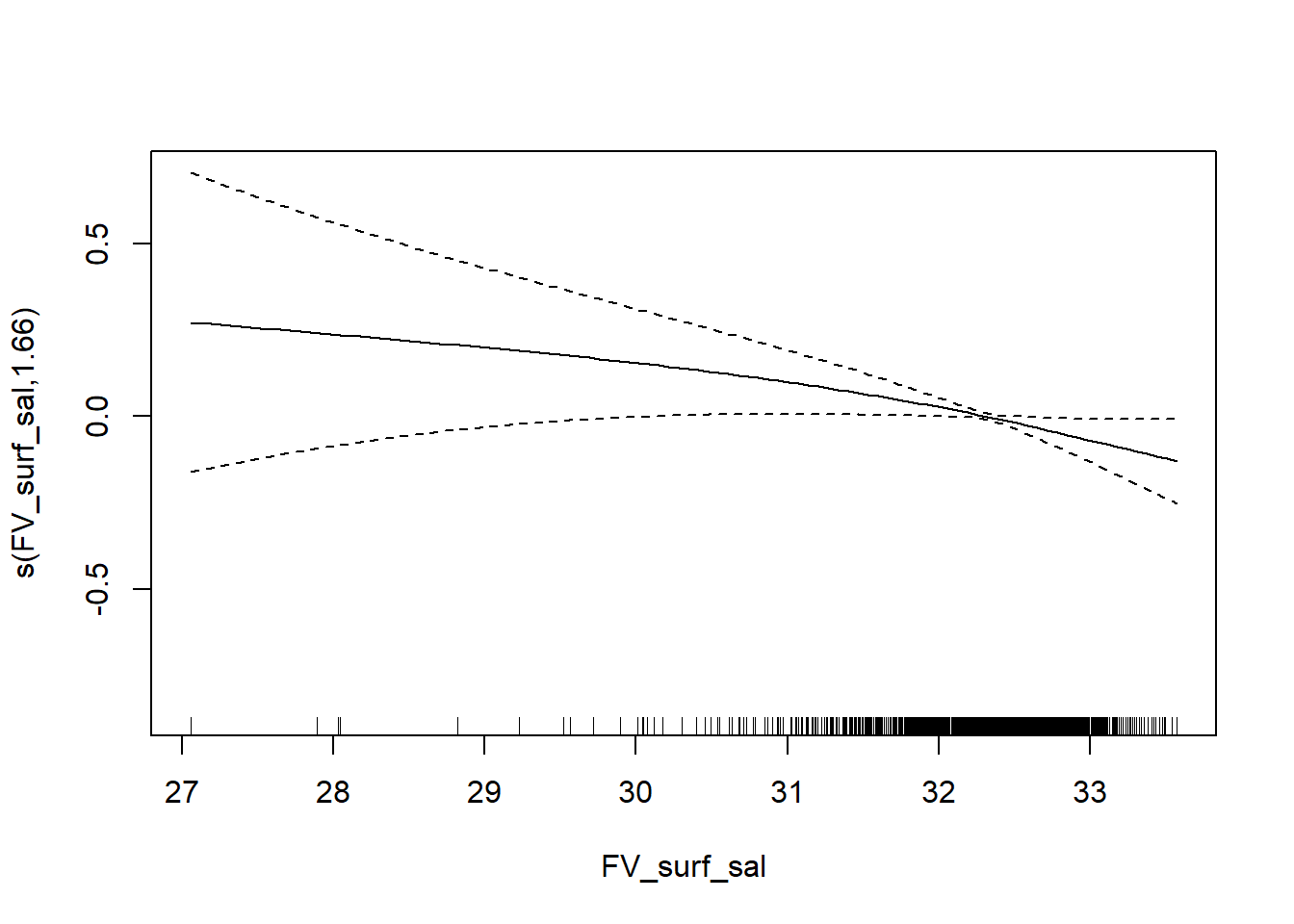
plot(N_Fall_FV$gam)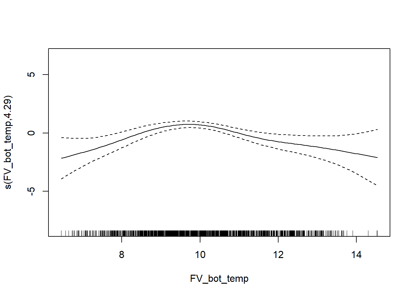
Shannon-Weiner Diversity
survey environmental data
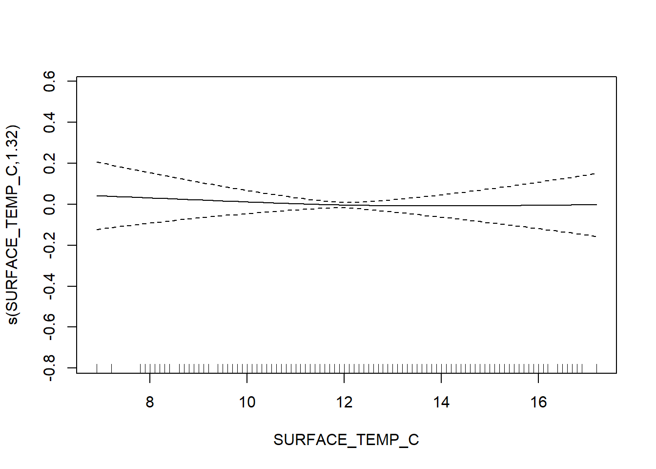
H_Fall <-  gamm4(H_index ~ s(WATER_TEMP_C) + s(SURFACE_TEMP_C) + s(SALINITY) + s(SURFACE_SALINITY) + s(START_DEPTH)+ s(START_LATITUDE, START_LONGITUDE) + s(metric_tons), random = ~ (1|YEAR), data = fall)

gam.check(H_Fall$gam)
##
## 'gamm' based fit - care required with interpretation.
## Checks based on working residuals may be misleading.
## Basis dimension (k) checking results. Low p-value (k-index<1) may
## indicate that k is too low, especially if edf is close to k'.
##
## k' edf k-index p-value
## s(WATER_TEMP_C) 9.00 3.21 0.95 0.020 *
## s(SURFACE_TEMP_C) 9.00 1.32 0.98 0.150
## s(SALINITY) 9.00 1.23 0.96 0.045 *
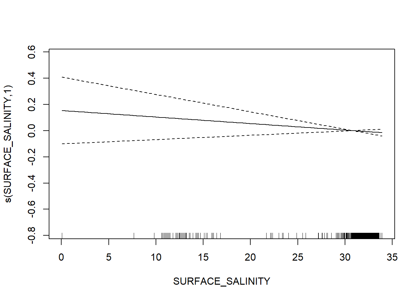
## s(SURFACE_SALINITY) 9.00 1.00 0.99 0.330
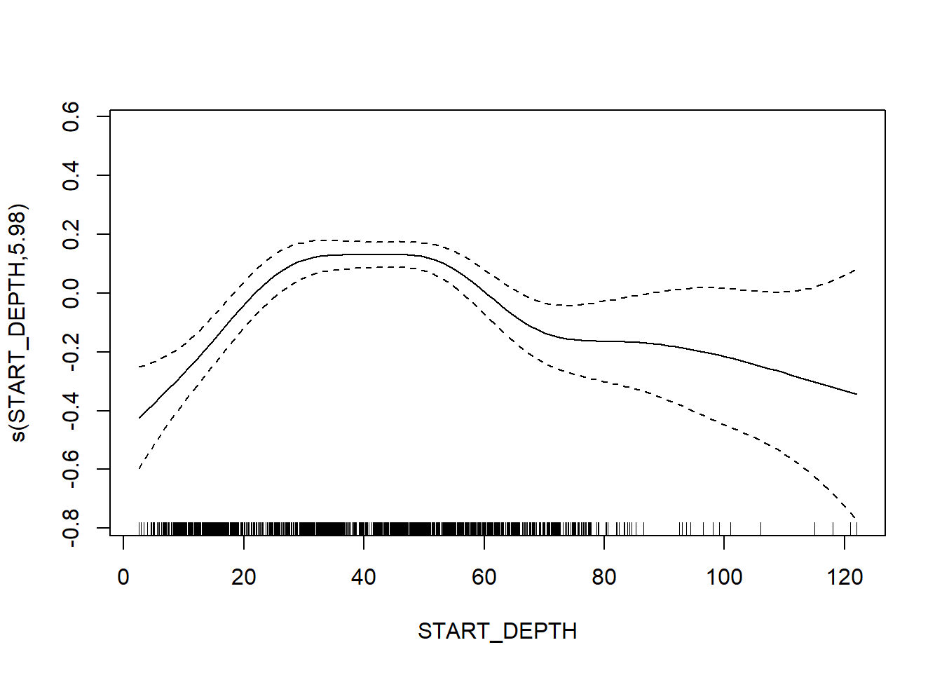
## s(START_DEPTH) 9.00 5.98 0.97 0.115
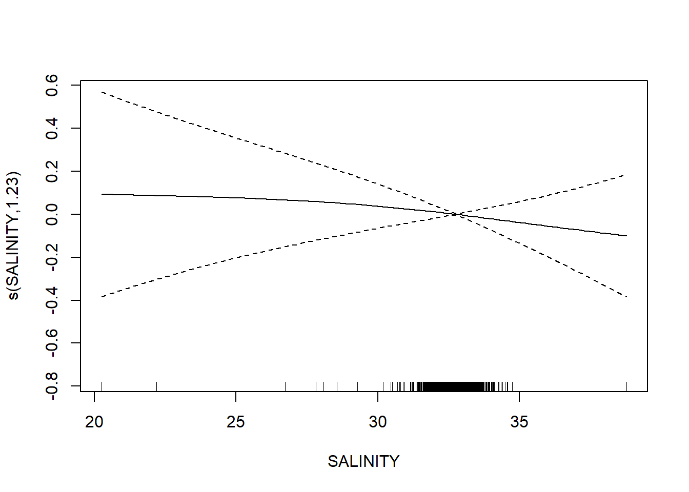
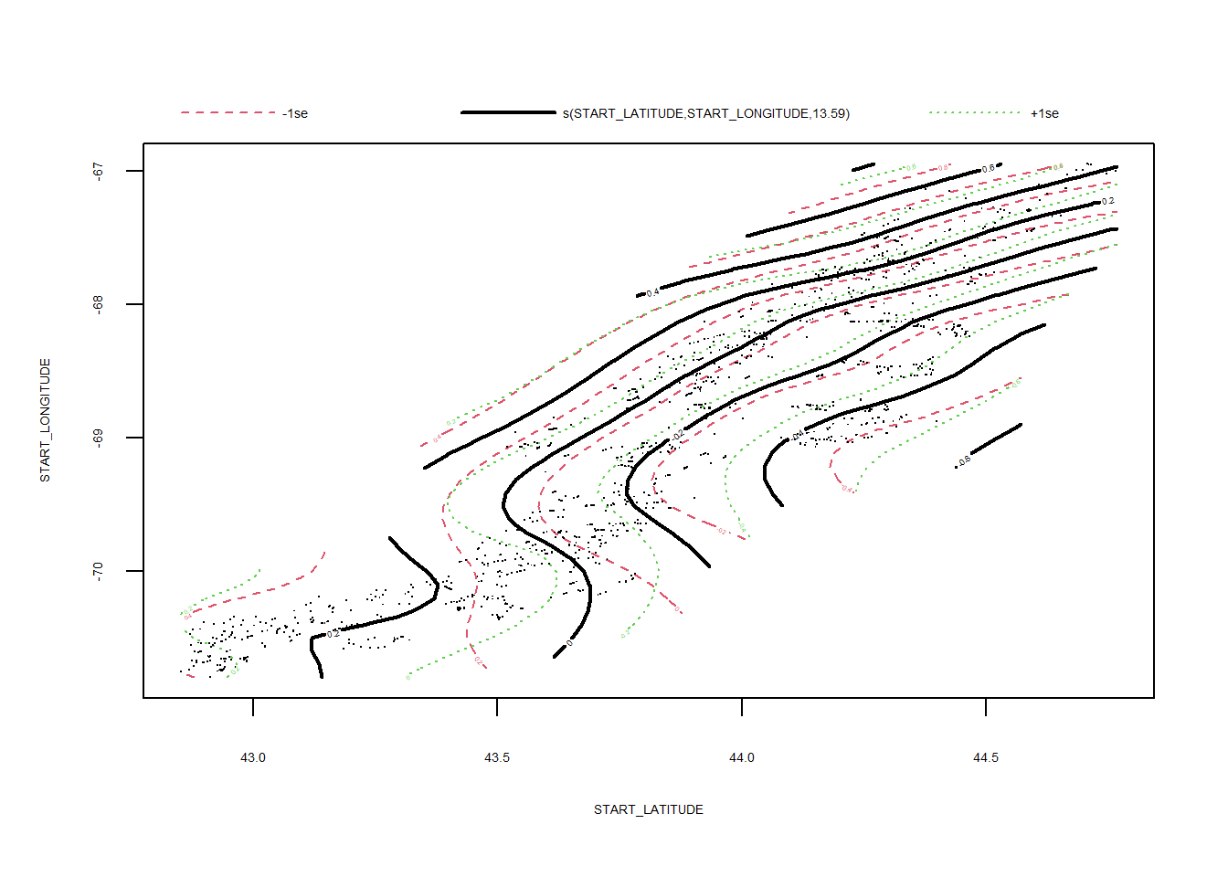
## s(START_LATITUDE,START_LONGITUDE) 29.00 13.59 1.00 0.440
## s(metric_tons) 9.00 1.00 0.91 0.005 **
## ---
## Signif. codes: 0 '***' 0.001 '**' 0.01 '*' 0.05 '.' 0.1 ' ' 1summary(H_Fall$gam)##
## Family: gaussian
## Link function: identity
##
## Formula:
## H_index ~ s(WATER_TEMP_C) + s(SURFACE_TEMP_C) + s(SALINITY) +
## s(SURFACE_SALINITY) + s(START_DEPTH) + s(START_LATITUDE,
## START_LONGITUDE) + s(metric_tons)
##
## Parametric coefficients:
## Estimate Std. Error t value Pr(>|t|)
## (Intercept) 1.46154 0.02486 58.79 <2e-16 ***
## ---
## Signif. codes: 0 '***' 0.001 '**' 0.01 '*' 0.05 '.' 0.1 ' ' 1
##
## Approximate significance of smooth terms:
## edf Ref.df F p-value
## s(WATER_TEMP_C) 3.209 3.209 4.688 0.00331 **
## s(SURFACE_TEMP_C) 1.323 1.323 0.070 0.80853
## s(SALINITY) 1.234 1.234 0.318 0.56127
## s(SURFACE_SALINITY) 1.000 1.000 1.451 0.22858
## s(START_DEPTH) 5.980 5.980 20.971 < 2e-16 ***
## s(START_LATITUDE,START_LONGITUDE) 13.592 13.592 19.210 < 2e-16 ***
## s(metric_tons) 1.000 1.000 0.177 0.67438
## ---
## Signif. codes: 0 '***' 0.001 '**' 0.01 '*' 0.05 '.' 0.1 ' ' 1
##
## R-sq.(adj) = 0.256
## lmer.REML = 1437.2 Scale est. = 0.1609 n = 1309plot(H_Fall$gam)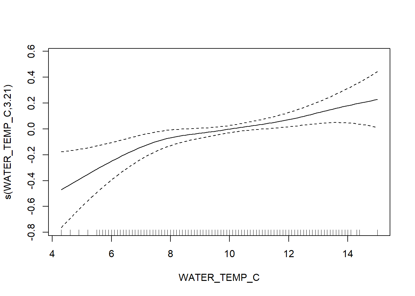
FVCOM data
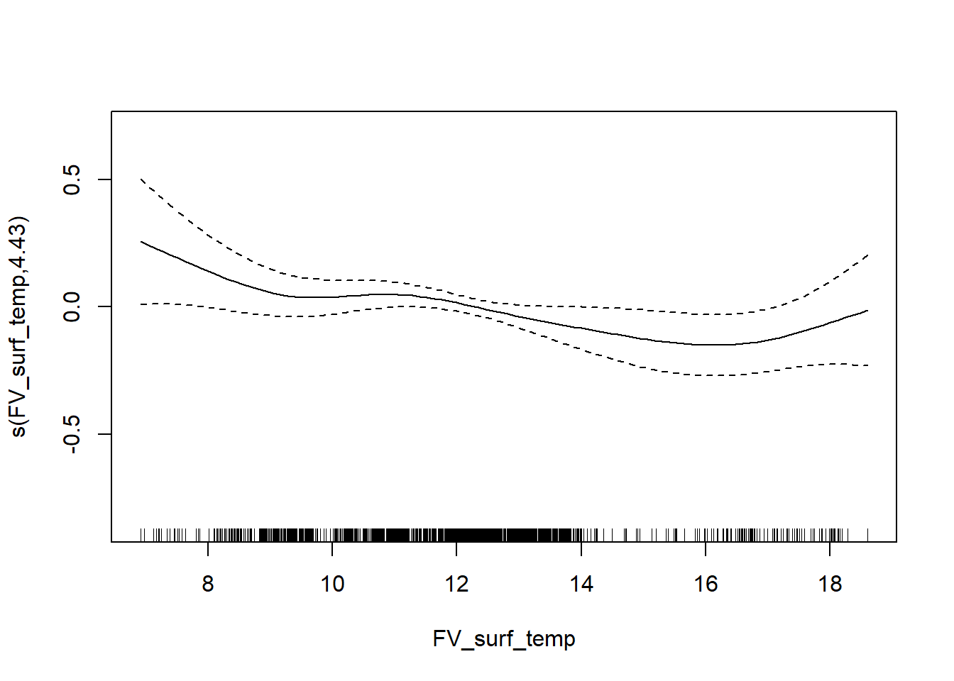
H_Fall_FV <- gamm4(H_index ~ s(FV_bot_temp) + s(FV_surf_temp) + s(FV_bot_sal) +  s(metric_tons) + s(FV_surf_sal) +  s(START_DEPTH) + s(START_LATITUDE, START_LONGITUDE), random = ~ (1|YEAR) , data = fall_fvcom)

gam.check(H_Fall_FV$gam)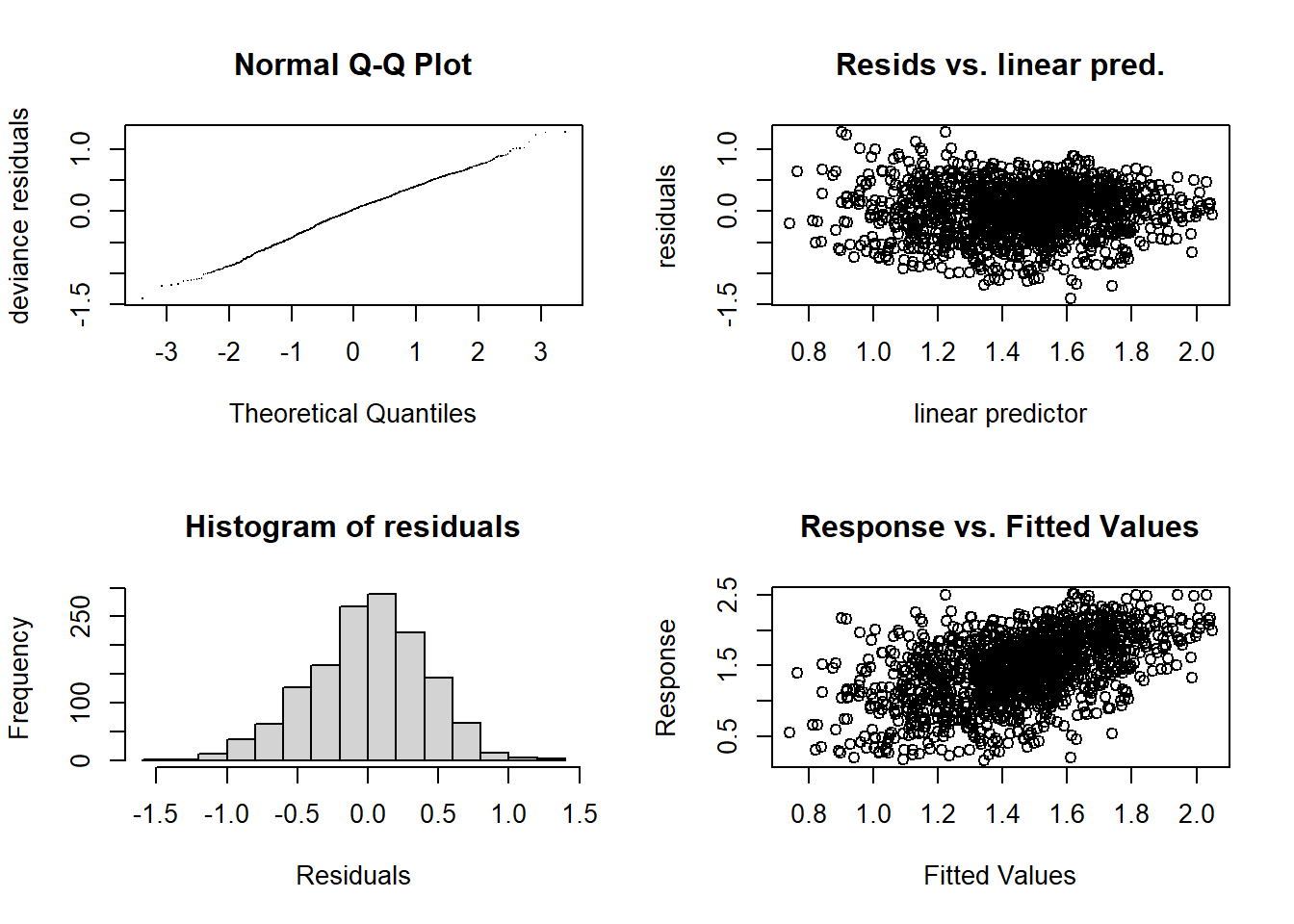
##
## 'gamm' based fit - care required with interpretation.
## Checks based on working residuals may be misleading.
## Basis dimension (k) checking results. Low p-value (k-index<1) may
## indicate that k is too low, especially if edf is close to k'.
##
## k' edf k-index p-value
## s(FV_bot_temp) 9.00 2.53 1.06 0.99
## s(FV_surf_temp) 9.00 4.43 0.93 <2e-16 ***
## s(FV_bot_sal) 9.00 1.00 1.01 0.61
## s(metric_tons) 9.00 1.00 0.91 <2e-16 ***
## s(FV_surf_sal) 9.00 1.66 0.99 0.30
## s(START_DEPTH) 9.00 5.88 0.99 0.40
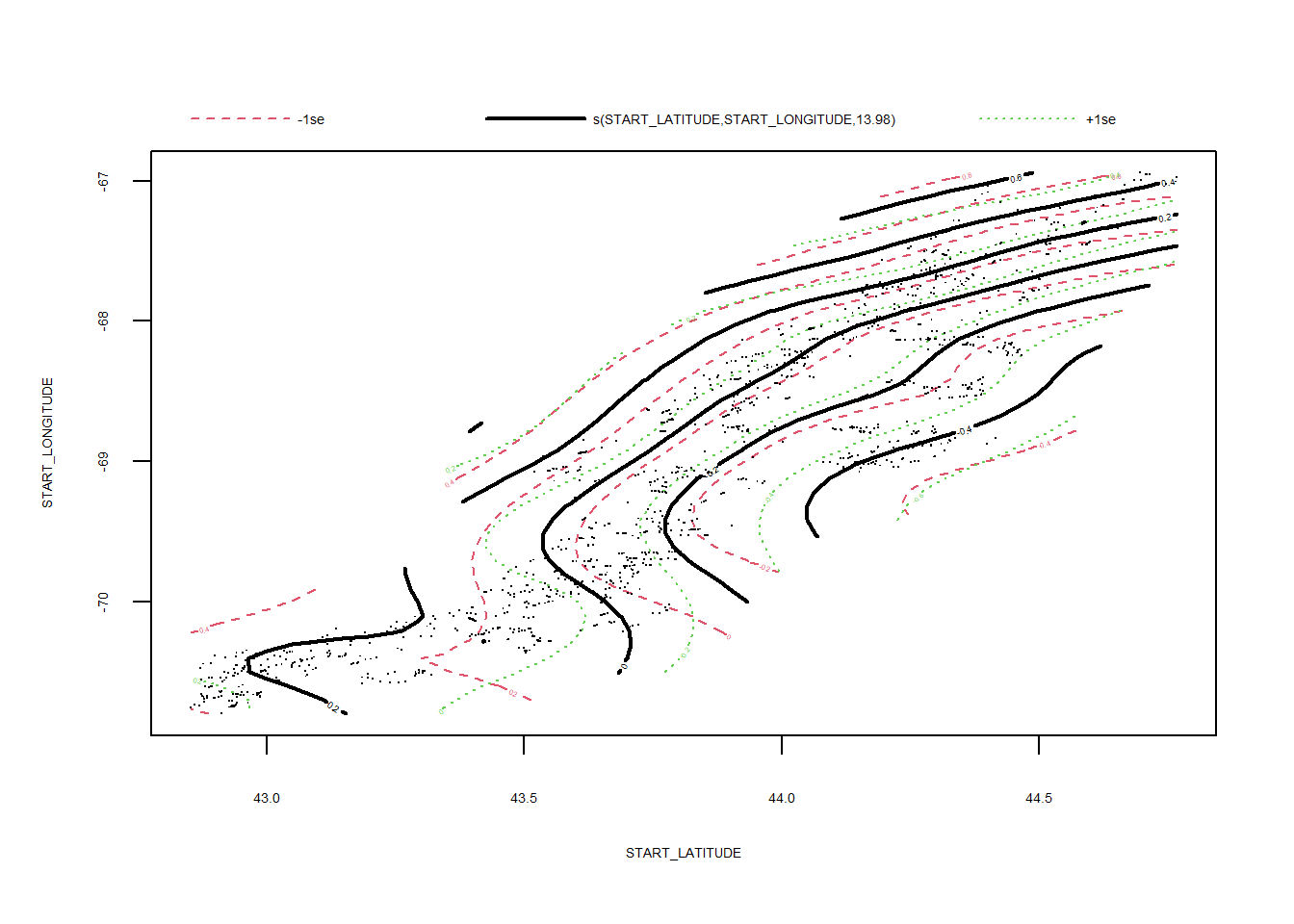
## s(START_LATITUDE,START_LONGITUDE) 29.00 13.98 1.00 0.54
## ---
## Signif. codes: 0 '***' 0.001 '**' 0.01 '*' 0.05 '.' 0.1 ' ' 1summary(H_Fall_FV$gam)##
## Family: gaussian
## Link function: identity
##
## Formula:
## H_index ~ s(FV_bot_temp) + s(FV_surf_temp) + s(FV_bot_sal) +
## s(metric_tons) + s(FV_surf_sal) + s(START_DEPTH) + s(START_LATITUDE,
## START_LONGITUDE)
##
## Parametric coefficients:
## Estimate Std. Error t value Pr(>|t|)
## (Intercept) 1.45553 0.02247 64.79 <2e-16 ***
## ---
## Signif. codes: 0 '***' 0.001 '**' 0.01 '*' 0.05 '.' 0.1 ' ' 1
##
## Approximate significance of smooth terms:
## edf Ref.df F p-value
## s(FV_bot_temp) 2.527 2.527 6.164 0.00231 **
## s(FV_surf_temp) 4.430 4.430 1.913 0.08483 .
## s(FV_bot_sal) 1.000 1.000 4.304 0.03822 *
## s(metric_tons) 1.000 1.000 0.000 0.99604
## s(FV_surf_sal) 1.661 1.661 2.672 0.05869 .
## s(START_DEPTH) 5.876 5.876 20.302 < 2e-16 ***
## s(START_LATITUDE,START_LONGITUDE) 13.981 13.981 14.581 < 2e-16 ***
## ---
## Signif. codes: 0 '***' 0.001 '**' 0.01 '*' 0.05 '.' 0.1 ' ' 1
##
## R-sq.(adj) = 0.241
## lmer.REML = 1596.1 Scale est. = 0.16608 n = 1417plot(H_Fall_FV$gam)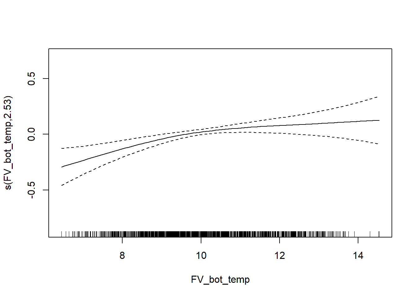
Simpson’s Diversity
survey environmental data
D_Fall <- gamm4(D_index  ~ s(WATER_TEMP_C) + s(SURFACE_TEMP_C) + s(SALINITY) +
                  s(SURFACE_SALINITY)  + s(START_DEPTH)+ s(START_LATITUDE, START_LONGITUDE) + s(metric_tons), random = ~ (1|YEAR), data = fall)

gam.check(D_Fall$gam)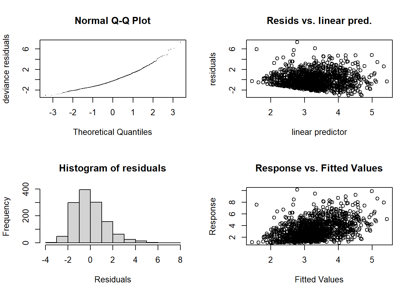
##
## 'gamm' based fit - care required with interpretation.
## Checks based on working residuals may be misleading.
## Basis dimension (k) checking results. Low p-value (k-index<1) may
## indicate that k is too low, especially if edf is close to k'.
##
##                                      k'   edf k-index p-value
## s(WATER_TEMP_C)                    9.00  1.00    0.97   0.145
## s(SURFACE_TEMP_C)                  9.00  1.15    0.96   0.095 .
## s(SALINITY)                        9.00  1.00    0.95   0.015 *
## s(SURFACE_SALINITY)                9.00  1.00    1.00   0.475
## s(START_DEPTH)                     9.00  5.80    0.98   0.225
## s(START_LATITUDE,START_LONGITUDE) 29.00 10.59    1.01   0.580
## s(metric_tons)                     9.00  1.00    0.90  <2e-16 ***
## ---
## Signif. codes: 0 '***' 0.001 '**' 0.01 '*' 0.05 '.' 0.1 ' ' 1summary(D_Fall$gam)##
## Family: gaussian
## Link function: identity
##
## Formula:
## D_index ~ s(WATER_TEMP_C) + s(SURFACE_TEMP_C) + s(SALINITY) +
## s(SURFACE_SALINITY) + s(START_DEPTH) + s(START_LATITUDE,
## START_LONGITUDE) + s(metric_tons)
##
## Parametric coefficients:
## Estimate Std. Error t value Pr(>|t|)
## (Intercept) 3.29958 0.08221 40.14 <2e-16 ***
## ---
## Signif. codes: 0 '***' 0.001 '**' 0.01 '*' 0.05 '.' 0.1 ' ' 1
##
## Approximate significance of smooth terms:
## edf Ref.df F p-value
## s(WATER_TEMP_C) 1.000 1.000 8.665 0.0033 **
## s(SURFACE_TEMP_C) 1.153 1.153 0.204 0.7954
## s(SALINITY) 1.000 1.000 0.028 0.8683
## s(SURFACE_SALINITY) 1.000 1.000 0.518 0.4719
## s(START_DEPTH) 5.802 5.802 12.784 <2e-16 ***
## s(START_LATITUDE,START_LONGITUDE) 10.585 10.585 17.479 <2e-16 ***
## s(metric_tons) 1.000 1.000 0.495 0.4818
## ---
## Signif. codes: 0 '***' 0.001 '**' 0.01 '*' 0.05 '.' 0.1 ' ' 1
##
## R-sq.(adj) = 0.171
## lmer.REML = 4643.5 Scale est. = 1.9157 n = 1309plot(D_Fall$gam)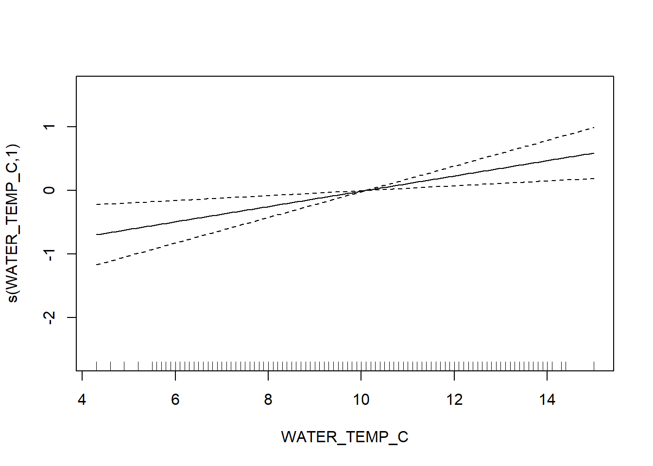
FVCOM data
D_Fall_FV <- gamm4(D_index ~ s(FV_bot_temp) + s(FV_surf_temp) + s(FV_bot_sal) +  s(metric_tons) +s(FV_surf_sal) +  s(START_DEPTH) + s(START_LATITUDE, START_LONGITUDE), random = ~ (1|YEAR) , data = fall_fvcom)

gam.check(D_Fall_FV$gam)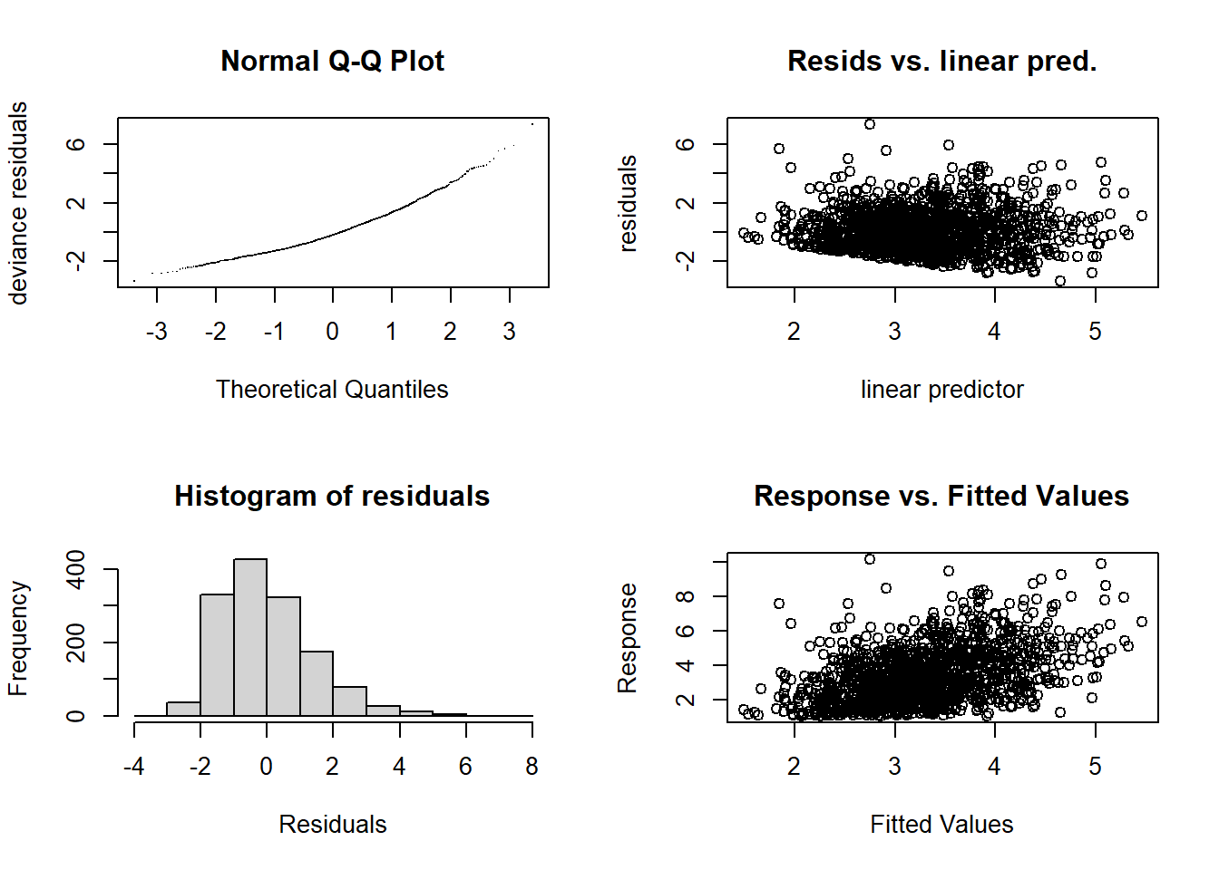
##
## 'gamm' based fit - care required with interpretation.
## Checks based on working residuals may be misleading.
## Basis dimension (k) checking results. Low p-value (k-index<1) may
## indicate that k is too low, especially if edf is close to k'.
##
##                                      k'   edf k-index p-value
## s(FV_bot_temp)                     9.00  1.60    1.06   0.970
## s(FV_surf_temp)                    9.00  5.55    0.96   0.065 .
## s(FV_bot_sal)                      9.00  1.00    1.01   0.655
## s(metric_tons)                     9.00  1.00    0.91  <2e-16 ***
## s(FV_surf_sal)                     9.00  1.41    0.97   0.145
## s(START_DEPTH)                     9.00  6.31    1.01   0.575
## s(START_LATITUDE,START_LONGITUDE) 29.00 11.72    1.00   0.395
## ---
## Signif. codes: 0 '***' 0.001 '**' 0.01 '*' 0.05 '.' 0.1 ' ' 1summary(D_Fall_FV$gam)##
## Family: gaussian
## Link function: identity
##
## Formula:
## D_index ~ s(FV_bot_temp) + s(FV_surf_temp) + s(FV_bot_sal) +
## s(metric_tons) + s(FV_surf_sal) + s(START_DEPTH) + s(START_LATITUDE,
## START_LONGITUDE)
##
## Parametric coefficients:
## Estimate Std. Error t value Pr(>|t|)
## (Intercept) 3.27804 0.06846 47.88 <2e-16 ***
## ---
## Signif. codes: 0 '***' 0.001 '**' 0.01 '*' 0.05 '.' 0.1 ' ' 1
##
## Approximate significance of smooth terms:
## edf Ref.df F p-value
## s(FV_bot_temp) 1.599 1.599 2.390 0.0599 .
## s(FV_surf_temp) 5.552 5.552 2.204 0.0511 .
## s(FV_bot_sal) 1.000 1.000 2.453 0.1176
## s(metric_tons) 1.000 1.000 0.175 0.6761
## s(FV_surf_sal) 1.408 1.408 1.182 0.2221
## s(START_DEPTH) 6.312 6.312 11.395 <2e-16 ***
## s(START_LATITUDE,START_LONGITUDE) 11.717 11.717 13.127 <2e-16 ***
## ---
## Signif. codes: 0 '***' 0.001 '**' 0.01 '*' 0.05 '.' 0.1 ' ' 1
##
## R-sq.(adj) = 0.179
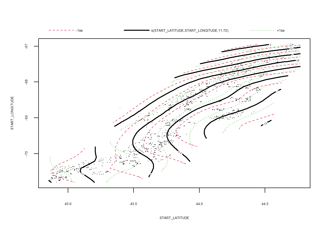
## lmer.REML = 5041.1 Scale est. = 1.9254 n = 1417plot(D_Fall_FV$gam)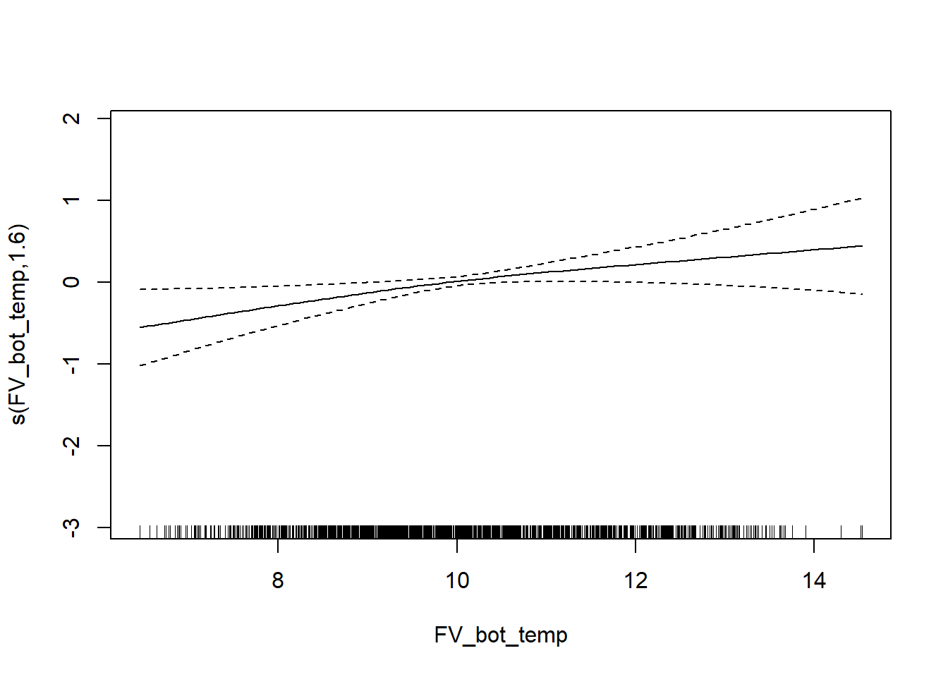
Simpson’s Evenness
survey environmental data
E_Fall <- gamm4(E_index  ~ s(WATER_TEMP_C) + s(SURFACE_TEMP_C) + s(SALINITY) +  s(SURFACE_SALINITY) + s(START_DEPTH)+ s(START_LATITUDE, START_LONGITUDE) + s(metric_tons), random = ~ (1|YEAR), data = fall)

gam.check(E_Fall$gam)
##
## 'gamm' based fit - care required with interpretation.
## Checks based on working residuals may be misleading.
## Basis dimension (k) checking results. Low p-value (k-index<1) may
## indicate that k is too low, especially if edf is close to k'.
##
##                                      k'   edf k-index p-value
## s(WATER_TEMP_C)                    9.00  1.00    0.99   0.345
## s(SURFACE_TEMP_C)                  9.00  1.00    0.99   0.250
## s(SALINITY)                        9.00  1.00    0.95   0.065 .
## s(SURFACE_SALINITY)                9.00  1.13    0.98   0.255
## s(START_DEPTH)                     9.00  3.69    0.98   0.260
## s(START_LATITUDE,START_LONGITUDE) 29.00  8.92    0.97   0.100 .
## s(metric_tons)                     9.00  1.00    0.94   0.005 **
## ---
## Signif. codes: 0 '***' 0.001 '**' 0.01 '*' 0.05 '.' 0.1 ' ' 1summary(E_Fall$gam)##
## Family: gaussian
## Link function: identity
##
## Formula:
## E_index ~ s(WATER_TEMP_C) + s(SURFACE_TEMP_C) + s(SALINITY) +
## s(SURFACE_SALINITY) + s(START_DEPTH) + s(START_LATITUDE,
## START_LONGITUDE) + s(metric_tons)
##
## Parametric coefficients:
## Estimate Std. Error t value Pr(>|t|)
## (Intercept) 0.158911 0.003663 43.39 <2e-16 ***
## ---
## Signif. codes: 0 '***' 0.001 '**' 0.01 '*' 0.05 '.' 0.1 ' ' 1
##
## Approximate significance of smooth terms:
## edf Ref.df F p-value
## s(WATER_TEMP_C) 1.000 1.000 15.023 0.000112 ***
## s(SURFACE_TEMP_C) 1.000 1.000 0.000 0.983045
## s(SALINITY) 1.000 1.000 1.081 0.298705
## s(SURFACE_SALINITY) 1.132 1.132 0.008 0.957530
## s(START_DEPTH) 3.686 3.686 3.457 0.008991 **
## s(START_LATITUDE,START_LONGITUDE) 8.924 8.924 13.060 < 2e-16 ***
## s(metric_tons) 1.000 1.000 1.352 0.245098
## ---
## Signif. codes: 0 '***' 0.001 '**' 0.01 '*' 0.05 '.' 0.1 ' ' 1
##
## R-sq.(adj) = 0.117
## lmer.REML = -3109.4 Scale est. = 0.0049795 n = 1309plot(E_Fall$gam)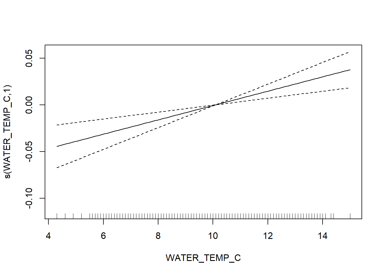
FVCOM data
E_Fall_FV <- gamm4(E_index ~ s(FV_bot_temp) + s(FV_surf_temp) + s(FV_bot_sal) +  s(metric_tons) + s(FV_surf_sal) +  s(START_DEPTH) + s(START_LATITUDE, START_LONGITUDE), random = ~ (1|YEAR) , data = fall_fvcom)

gam.check(E_Fall_FV$gam)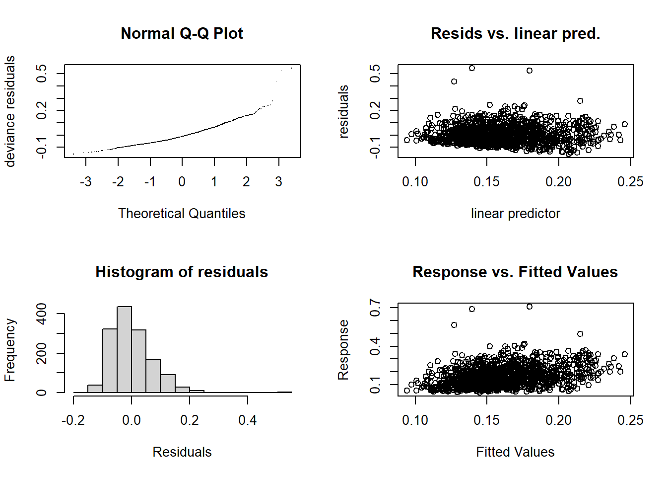
##
## 'gamm' based fit - care required with interpretation.
## Checks based on working residuals may be misleading.
## Basis dimension (k) checking results. Low p-value (k-index<1) may
## indicate that k is too low, especially if edf is close to k'.
##
##                                      k'   edf k-index p-value
## s(FV_bot_temp)                     9.00  1.00    1.06    1.00
## s(FV_surf_temp)                    9.00  1.00    0.95    0.02 *
## s(FV_bot_sal)                      9.00  1.70    1.01    0.62
## s(metric_tons)                     9.00  1.00    0.94    0.01 **
## s(FV_surf_sal)                     9.00  1.00    1.01    0.60
## s(START_DEPTH)                     9.00  4.02    1.00    0.43
## s(START_LATITUDE,START_LONGITUDE) 29.00  9.87    0.97    0.13
## ---
## Signif. codes: 0 '***' 0.001 '**' 0.01 '*' 0.05 '.' 0.1 ' ' 1summary(E_Fall_FV$gam)##
## Family: gaussian
## Link function: identity
##
## Formula:
## E_index ~ s(FV_bot_temp) + s(FV_surf_temp) + s(FV_bot_sal) +
## s(metric_tons) + s(FV_surf_sal) + s(START_DEPTH) + s(START_LATITUDE,
## START_LONGITUDE)
##
## Parametric coefficients:
## Estimate Std. Error t value Pr(>|t|)
## (Intercept) 0.158785 0.003012 52.71 <2e-16 ***
## ---
## Signif. codes: 0 '***' 0.001 '**' 0.01 '*' 0.05 '.' 0.1 ' ' 1
##
## Approximate significance of smooth terms:
## edf Ref.df F p-value
## s(FV_bot_temp) 1.000 1.000 10.044 0.00156 **
## s(FV_surf_temp) 1.000 1.000 1.598 0.20638
## s(FV_bot_sal) 1.702 1.702 2.603 0.16577
## s(metric_tons) 1.000 1.000 1.527 0.21675
## s(FV_surf_sal) 1.000 1.000 2.245 0.13424
## s(START_DEPTH) 4.020 4.020 3.960 0.00333 **
## s(START_LATITUDE,START_LONGITUDE) 9.872 9.872 10.925 < 2e-16 ***
## ---
## Signif. codes: 0 '***' 0.001 '**' 0.01 '*' 0.05 '.' 0.1 ' ' 1
##
## R-sq.(adj) = 0.12
## lmer.REML = -3374.5 Scale est. = 0.0049853 n = 1417plot(E_Fall_FV$gam)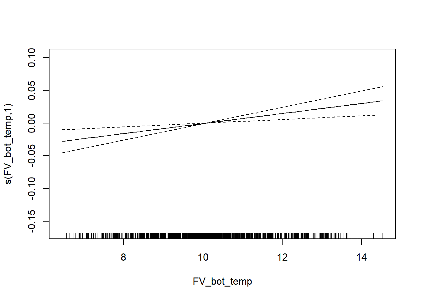
Taxonomic diversity
survey environmental data
delta_Fall <- gamm4(delta ~ s(WATER_TEMP_C) + s(SURFACE_TEMP_C) + s(SALINITY) + s(SURFACE_SALINITY) + s(START_DEPTH)+ s(START_LATITUDE, START_LONGITUDE) +  s(metric_tons), random = ~ (1|YEAR), data = fall)

gam.check(delta_Fall$gam)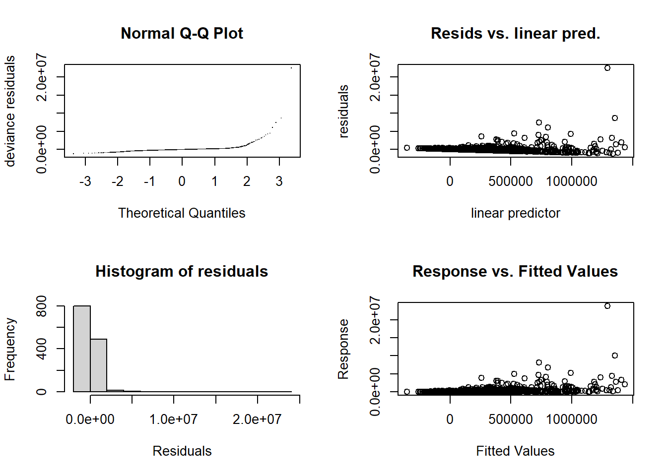
##
## 'gamm' based fit - care required with interpretation.
## Checks based on working residuals may be misleading.
## Basis dimension (k) checking results. Low p-value (k-index<1) may
## indicate that k is too low, especially if edf is close to k'.
##
##                                      k'   edf k-index p-value
## s(WATER_TEMP_C)                    9.00  1.86    0.98   0.140
## s(SURFACE_TEMP_C)                  9.00  1.00    1.00   0.475
## s(SALINITY)                        9.00  1.00    0.99   0.190
## s(SURFACE_SALINITY)                9.00  1.00    0.99   0.175
## s(START_DEPTH)                     9.00  4.90    1.01   0.595
## s(START_LATITUDE,START_LONGITUDE) 29.00 16.09    0.71   0.005 **
## s(metric_tons)                     9.00  4.25    0.97   0.065 .
## ---
## Signif. codes: 0 '***' 0.001 '**' 0.01 '*' 0.05 '.' 0.1 ' ' 1summary(delta_Fall$gam)##
## Family: gaussian
## Link function: identity
##
## Formula:
## delta ~ s(WATER_TEMP_C) + s(SURFACE_TEMP_C) + s(SALINITY) + s(SURFACE_SALINITY) +
## s(START_DEPTH) + s(START_LATITUDE, START_LONGITUDE) + s(metric_tons)
##
## Parametric coefficients:
## Estimate Std. Error t value Pr(>|t|)
## (Intercept) 245230 23935 10.25 <2e-16 ***
## ---
## Signif. codes: 0 '***' 0.001 '**' 0.01 '*' 0.05 '.' 0.1 ' ' 1
##
## Approximate significance of smooth terms:
## edf Ref.df F p-value
## s(WATER_TEMP_C) 1.858 1.858 0.764 0.465094
## s(SURFACE_TEMP_C) 1.000 1.000 0.002 0.963894
## s(SALINITY) 1.000 1.000 0.000 0.996332
## s(SURFACE_SALINITY) 1.000 1.000 0.323 0.570045
## s(START_DEPTH) 4.903 4.903 2.616 0.050604 .
## s(START_LATITUDE,START_LONGITUDE) 16.093 16.093 4.225 < 2e-16 ***
## s(metric_tons) 4.246 4.246 4.367 0.000819 ***
## ---
## Signif. codes: 0 '***' 0.001 '**' 0.01 '*' 0.05 '.' 0.1 ' ' 1
##
## R-sq.(adj) = 0.114
## lmer.REML = 39345 Scale est. = 7.4988e+11 n = 1309plot(delta_Fall$gam)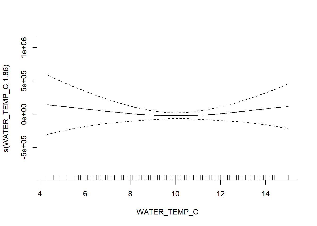
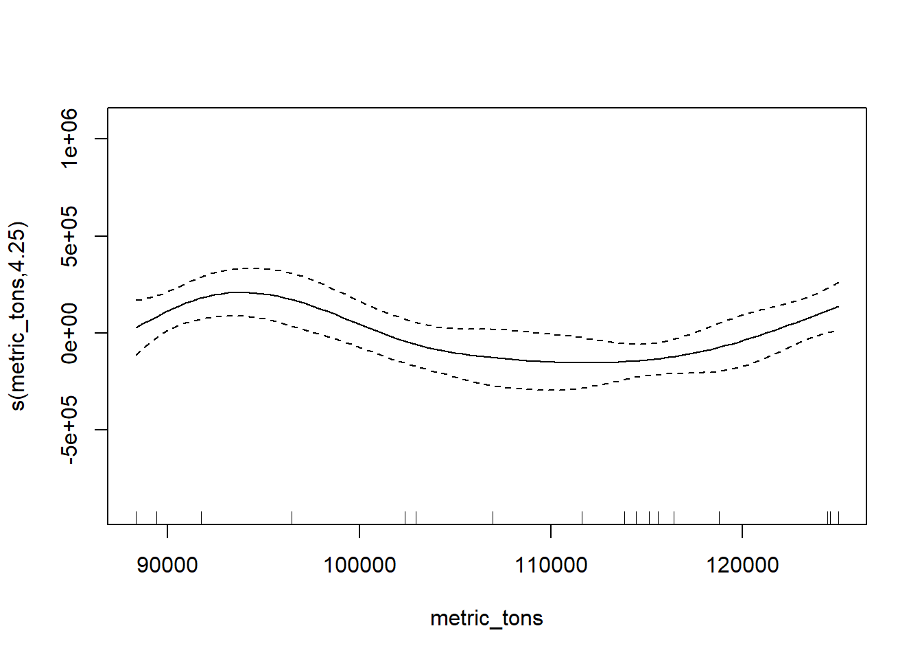
FVCOM data
delta_Fall_FV <- gamm4(delta ~ s(FV_bot_temp) + s(FV_surf_temp) + s(FV_bot_sal) +  s(metric_tons) +s(FV_surf_sal) +  s(START_DEPTH) + s(START_LATITUDE, START_LONGITUDE), random = ~ (1|YEAR) , data = fall_fvcom)

gam.check(delta_Fall_FV$gam)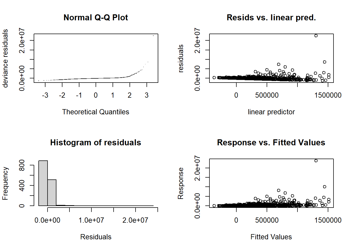
##
## 'gamm' based fit - care required with interpretation.
## Checks based on working residuals may be misleading.
## Basis dimension (k) checking results. Low p-value (k-index<1) may
## indicate that k is too low, especially if edf is close to k'.
##
##                                      k'   edf k-index p-value
## s(FV_bot_temp)                     9.00  2.89    1.03   0.975
## s(FV_surf_temp)                    9.00  1.13    1.00   0.320
## s(FV_bot_sal)                      9.00  1.00    0.98   0.090 .
## s(metric_tons)                     9.00  3.32    0.97   0.035 *
## s(FV_surf_sal)                     9.00  1.00    0.99   0.225
## s(START_DEPTH)                     9.00  5.15    1.00   0.485
## s(START_LATITUDE,START_LONGITUDE) 29.00 17.33    0.70  <2e-16 ***
## ---
## Signif. codes: 0 '***' 0.001 '**' 0.01 '*' 0.05 '.' 0.1 ' ' 1summary(delta_Fall_FV$gam)##
## Family: gaussian
## Link function: identity
##
## Formula:
## delta ~ s(FV_bot_temp) + s(FV_surf_temp) + s(FV_bot_sal) + s(metric_tons) +
## s(FV_surf_sal) + s(START_DEPTH) + s(START_LATITUDE, START_LONGITUDE)
##
## Parametric coefficients:
## Estimate Std. Error t value Pr(>|t|)
## (Intercept) 232132 26755 8.676 <2e-16 ***
## ---
## Signif. codes: 0 '***' 0.001 '**' 0.01 '*' 0.05 '.' 0.1 ' ' 1
##
## Approximate significance of smooth terms:
## edf Ref.df F p-value
## s(FV_bot_temp) 2.890 2.890 3.510 0.02483 *
## s(FV_surf_temp) 1.133 1.133 0.037 0.87560
## s(FV_bot_sal) 1.000 1.000 1.172 0.27919
## s(metric_tons) 3.321 3.321 4.409 0.00454 **
## s(FV_surf_sal) 1.000 1.000 0.726 0.39427
## s(START_DEPTH) 5.149 5.149 3.119 0.01345 *
## s(START_LATITUDE,START_LONGITUDE) 17.332 17.332 3.890 9.04e-07 ***
## ---
## Signif. codes: 0 '***' 0.001 '**' 0.01 '*' 0.05 '.' 0.1 ' ' 1
##
## R-sq.(adj) = 0.118
## lmer.REML = 42494 Scale est. = 6.8927e+11 n = 1417plot(delta_Fall_FV$gam)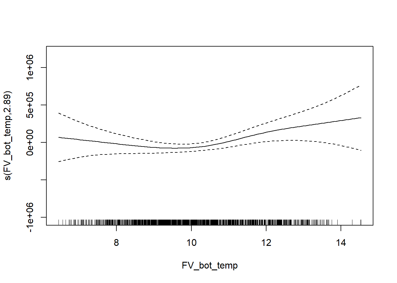
Taxonomic distinctness
survey environmental data
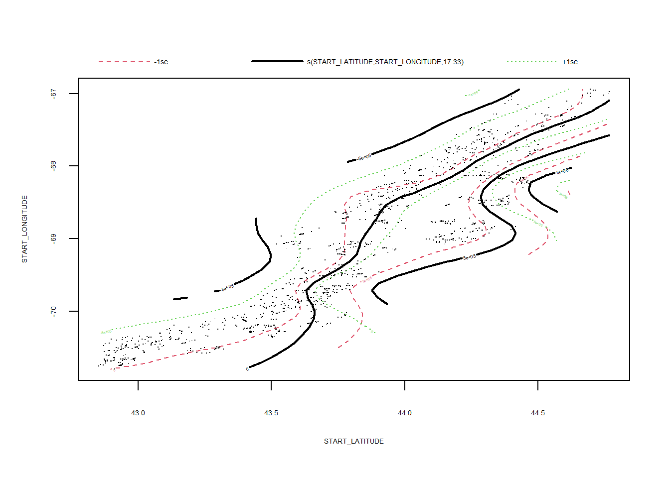
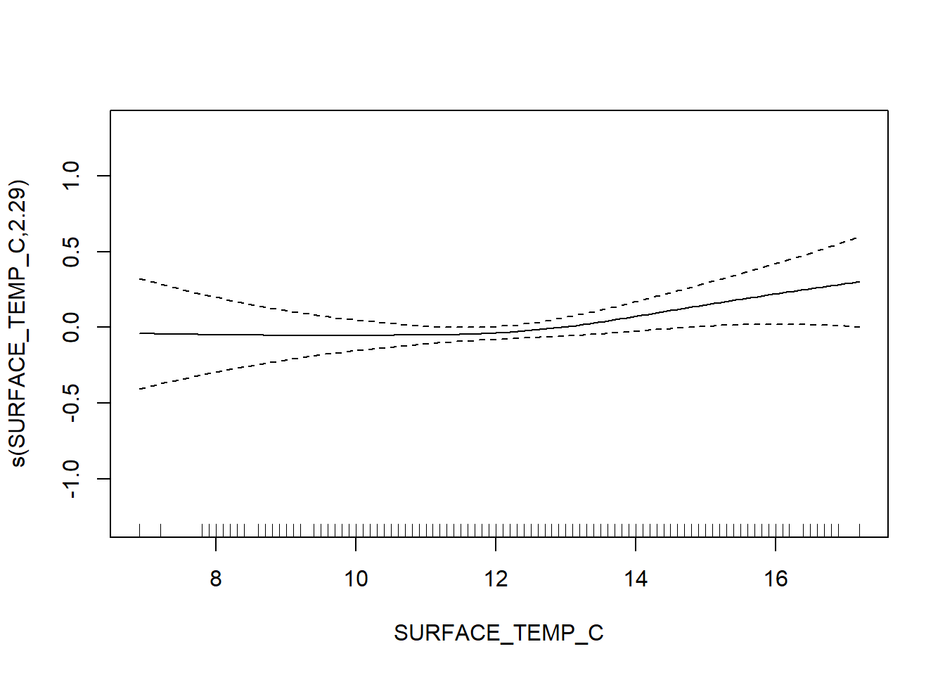
delta_star_Fall <- gamm4(delta_star ~ s(WATER_TEMP_C) + s(SURFACE_TEMP_C) + s(SALINITY) +  s(SURFACE_SALINITY) + s(START_DEPTH)+ s(START_LATITUDE, START_LONGITUDE) +  s(metric_tons), random = ~ (1|YEAR), data = fall)

gam.check(delta_star_Fall$gam)
##
## 'gamm' based fit - care required with interpretation.
## Checks based on working residuals may be misleading.
## Basis dimension (k) checking results. Low p-value (k-index<1) may
## indicate that k is too low, especially if edf is close to k'.
##
##                                      k'   edf k-index p-value
## s(WATER_TEMP_C)                    9.00  4.02    0.89  <2e-16 ***
## s(SURFACE_TEMP_C)                  9.00  2.29    0.94   0.010 **
## s(SALINITY)                        9.00  3.61    0.94   0.025 *
## s(SURFACE_SALINITY)                9.00  1.45    0.98   0.290
## s(START_DEPTH)                     9.00  4.32    0.99   0.320
## s(START_LATITUDE,START_LONGITUDE) 29.00 22.09    0.95   0.015 *
## s(metric_tons)                     9.00  1.44    0.82  <2e-16 ***
## ---
## Signif. codes: 0 '***' 0.001 '**' 0.01 '*' 0.05 '.' 0.1 ' ' 1summary(delta_star_Fall$gam)##
## Family: gaussian
## Link function: identity
##
## Formula:
## delta_star ~ s(WATER_TEMP_C) + s(SURFACE_TEMP_C) + s(SALINITY) +
## s(SURFACE_SALINITY) + s(START_DEPTH) + s(START_LATITUDE,
## START_LONGITUDE) + s(metric_tons)
##
## Parametric coefficients:
## Estimate Std. Error t value Pr(>|t|)
## (Intercept) 4.74975 0.04438 107 <2e-16 ***
## ---
## Signif. codes: 0 '***' 0.001 '**' 0.01 '*' 0.05 '.' 0.1 ' ' 1
##
## Approximate significance of smooth terms:
## edf Ref.df F p-value
## s(WATER_TEMP_C) 4.016 4.016 3.190 0.012720 *
## s(SURFACE_TEMP_C) 2.286 2.286 2.472 0.066567 .
## s(SALINITY) 3.609 3.609 1.249 0.168039
## s(SURFACE_SALINITY) 1.445 1.445 3.780 0.100605
## s(START_DEPTH) 4.321 4.321 5.360 0.000201 ***
## s(START_LATITUDE,START_LONGITUDE) 22.087 22.087 8.312 < 2e-16 ***
## s(metric_tons) 1.444 1.444 0.404 0.466825
## ---
## Signif. codes: 0 '***' 0.001 '**' 0.01 '*' 0.05 '.' 0.1 ' ' 1
##
## R-sq.(adj) = 0.169
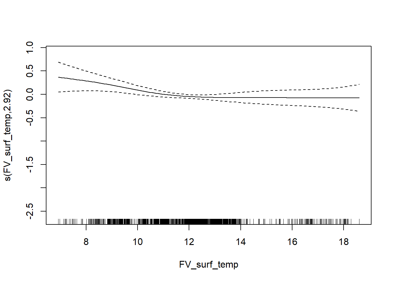
## lmer.REML = 2601.4 Scale est. = 0.38293 n = 1309plot(delta_star_Fall$gam)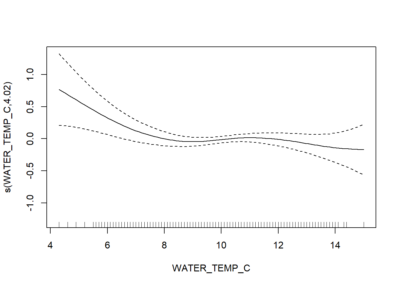
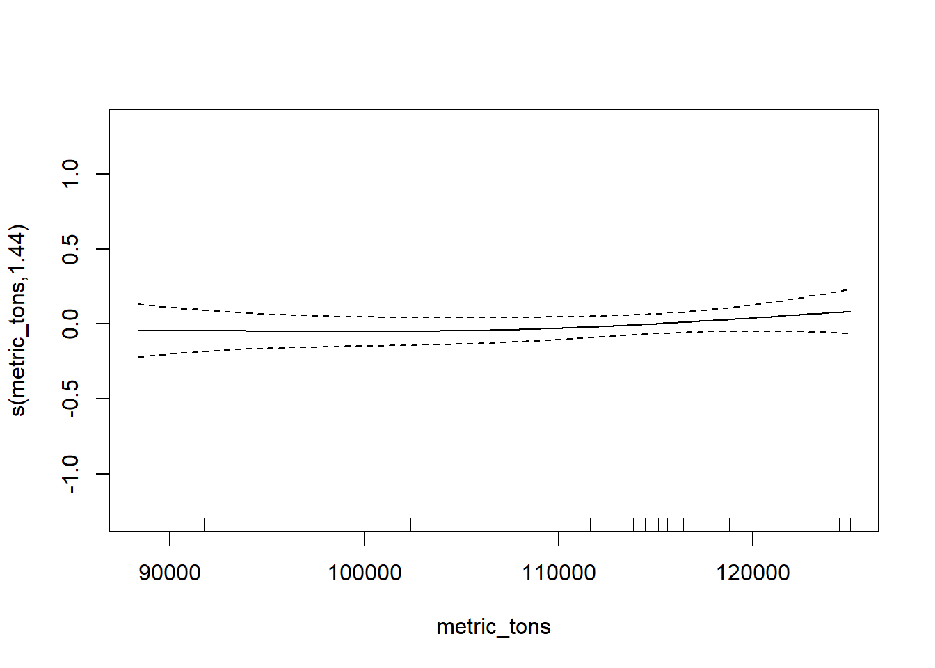
FVCOM data
delta_star_Fall_FV <- gamm4(delta_star ~ s(FV_bot_temp) + s(FV_surf_temp) + s(FV_bot_sal) +  s(metric_tons) + s(FV_surf_sal) +  s(START_DEPTH) + s(START_LATITUDE, START_LONGITUDE), random = ~ (1|YEAR) , data = fall_fvcom)

gam.check(delta_star_Fall_FV$gam)
##
## 'gamm' based fit - care required with interpretation.
## Checks based on working residuals may be misleading.
## Basis dimension (k) checking results. Low p-value (k-index<1) may
## indicate that k is too low, especially if edf is close to k'.
##
##                                      k'   edf k-index p-value
## s(FV_bot_temp)                     9.00  4.18    0.99   0.395
## s(FV_surf_temp)                    9.00  2.92    0.91  <2e-16 ***
## s(FV_bot_sal)                      9.00  5.23    1.01   0.720
## s(metric_tons)                     9.00  2.13    0.83  <2e-16 ***
## s(FV_surf_sal)                     9.00  2.15    1.02   0.715
## s(START_DEPTH)                     9.00  4.55    0.99   0.270
## s(START_LATITUDE,START_LONGITUDE) 29.00 20.33    0.96   0.015 *
## ---
## Signif. codes: 0 '***' 0.001 '**' 0.01 '*' 0.05 '.' 0.1 ' ' 1summary(delta_star_Fall_FV$gam)##
## Family: gaussian
## Link function: identity
##
## Formula:
## delta_star ~ s(FV_bot_temp) + s(FV_surf_temp) + s(FV_bot_sal) +
## s(metric_tons) + s(FV_surf_sal) + s(START_DEPTH) + s(START_LATITUDE,
## START_LONGITUDE)
##
## Parametric coefficients:
## Estimate Std. Error t value Pr(>|t|)
## (Intercept) 4.76615 0.03774 126.3 <2e-16 ***
## ---
## Signif. codes: 0 '***' 0.001 '**' 0.01 '*' 0.05 '.' 0.1 ' ' 1
##
## Approximate significance of smooth terms:
## edf Ref.df F p-value
## s(FV_bot_temp) 4.183 4.183 4.969 0.000695 ***
## s(FV_surf_temp) 2.921 2.921 3.265 0.030819 *
## s(FV_bot_sal) 5.227 5.227 4.128 0.000888 ***
## s(metric_tons) 2.131 2.131 1.803 0.147938
## s(FV_surf_sal) 2.147 2.147 1.010 0.390169
## s(START_DEPTH) 4.549 4.549 6.093 3.28e-05 ***
## s(START_LATITUDE,START_LONGITUDE) 20.329 20.329 6.194 < 2e-16 ***
## ---
## Signif. codes: 0 '***' 0.001 '**' 0.01 '*' 0.05 '.' 0.1 ' ' 1
##
## R-sq.(adj) = 0.18
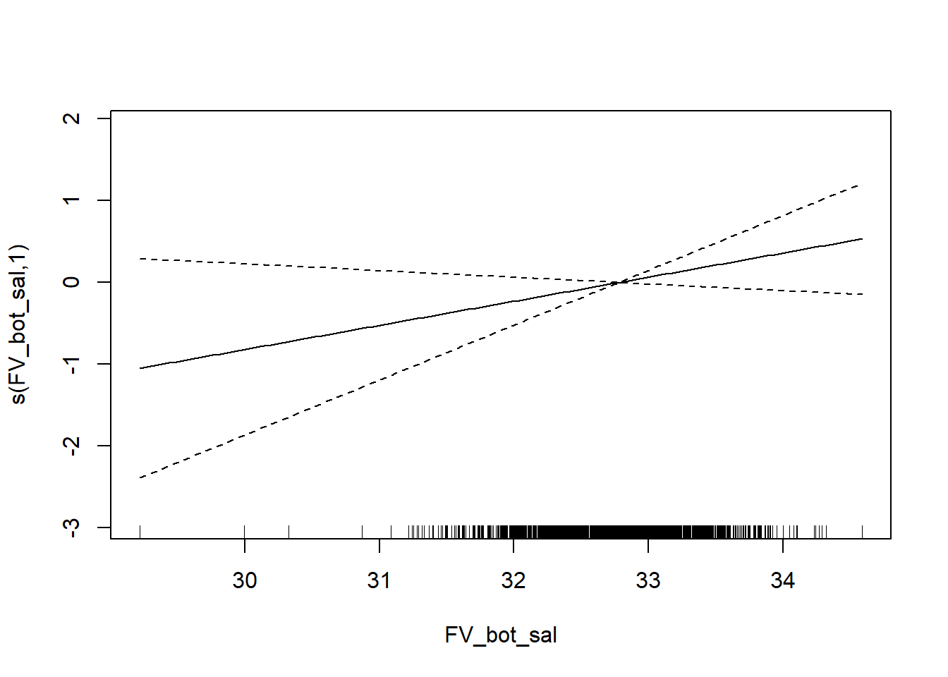
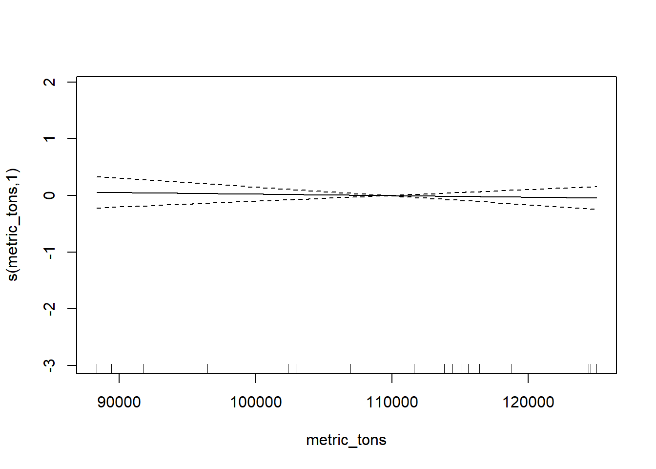
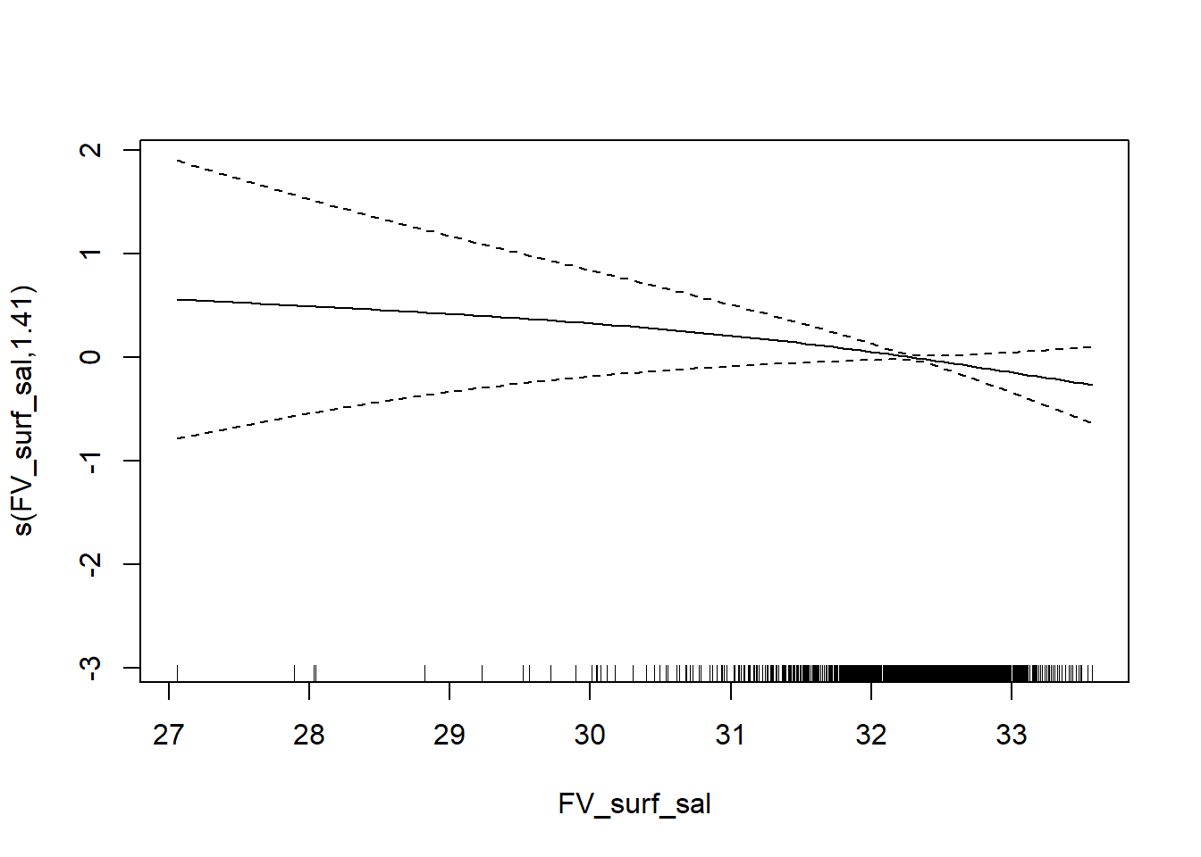
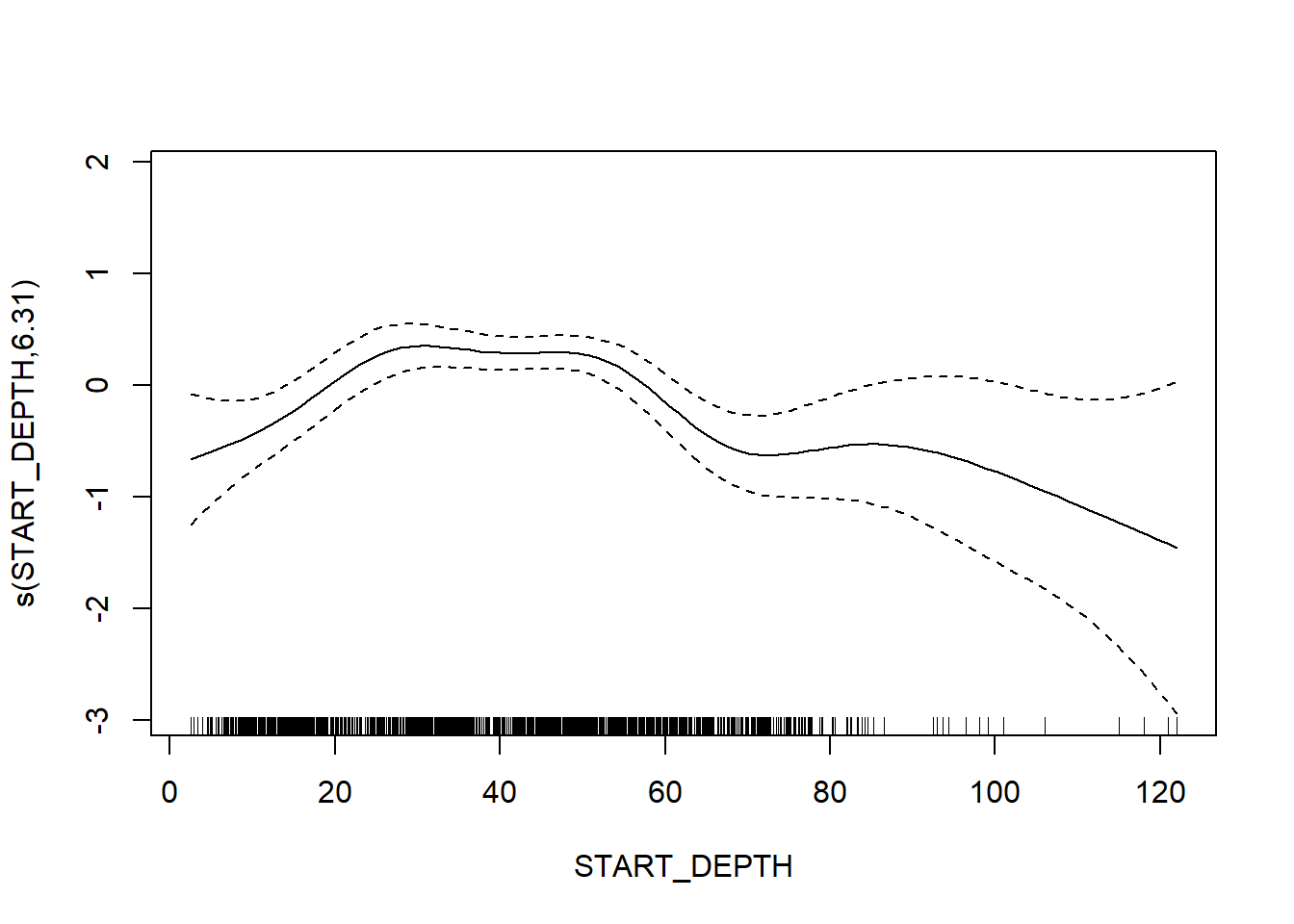
## lmer.REML = 2785.4 Scale est. = 0.37805 n = 1417plot(delta_star_Fall_FV$gam)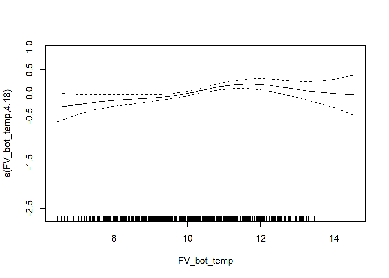
Average taxonomic distinctness
survey environmental data
delta_plus_Fall <- gamm4(delta_plus ~ s(WATER_TEMP_C) + s(SURFACE_TEMP_C) + s(SALINITY) +  s(SURFACE_SALINITY) + s(START_DEPTH)+ s(START_LATITUDE, START_LONGITUDE) +  s(metric_tons), random = ~ (1|YEAR), data = fall_fvcom)

gam.check(delta_plus_Fall$gam)
##
## 'gamm' based fit - care required with interpretation.
## Checks based on working residuals may be misleading.
## Basis dimension (k) checking results. Low p-value (k-index<1) may
## indicate that k is too low, especially if edf is close to k'.
##
##                                      k'   edf k-index p-value
## s(WATER_TEMP_C)                    9.00  2.05    0.90  <2e-16 ***
## s(SURFACE_TEMP_C)                  9.00  1.00    0.89  <2e-16 ***
## s(SALINITY)                        9.00  3.06    0.94    0.01 **
## s(SURFACE_SALINITY)                9.00  1.00    0.97    0.18
## s(START_DEPTH)                     9.00  5.39    1.03    0.84
## s(START_LATITUDE,START_LONGITUDE) 29.00  2.40    0.99    0.32
## s(metric_tons)                     9.00  1.64    0.77  <2e-16 ***
## ---
## Signif. codes: 0 '***' 0.001 '**' 0.01 '*' 0.05 '.' 0.1 ' ' 1summary(delta_plus_Fall$gam)##
## Family: gaussian
## Link function: identity
##
## Formula:
## delta_plus ~ s(WATER_TEMP_C) + s(SURFACE_TEMP_C) + s(SALINITY) +
## s(SURFACE_SALINITY) + s(START_DEPTH) + s(START_LATITUDE,
## START_LONGITUDE) + s(metric_tons)
##
## Parametric coefficients:
## Estimate Std. Error t value Pr(>|t|)
## (Intercept) 4.84587 0.01348 359.4 <2e-16 ***
## ---
## Signif. codes: 0 '***' 0.001 '**' 0.01 '*' 0.05 '.' 0.1 ' ' 1
##
## Approximate significance of smooth terms:
## edf Ref.df F p-value
## s(WATER_TEMP_C) 2.052 2.052 1.102 0.3718
## s(SURFACE_TEMP_C) 1.000 1.000 0.076 0.7832
## s(SALINITY) 3.065 3.065 2.565 0.0551 .
## s(SURFACE_SALINITY) 1.000 1.000 1.251 0.2636
## s(START_DEPTH) 5.389 5.389 10.986 < 2e-16 ***
## s(START_LATITUDE,START_LONGITUDE) 2.402 2.402 14.448 3.35e-07 ***
## s(metric_tons) 1.636 1.636 2.097 0.2535
## ---
## Signif. codes: 0 '***' 0.001 '**' 0.01 '*' 0.05 '.' 0.1 ' ' 1
##
## R-sq.(adj) = 0.115
## lmer.REML = -1064.8 Scale est. = 0.023743 n = 1309plot(delta_plus_Fall$gam)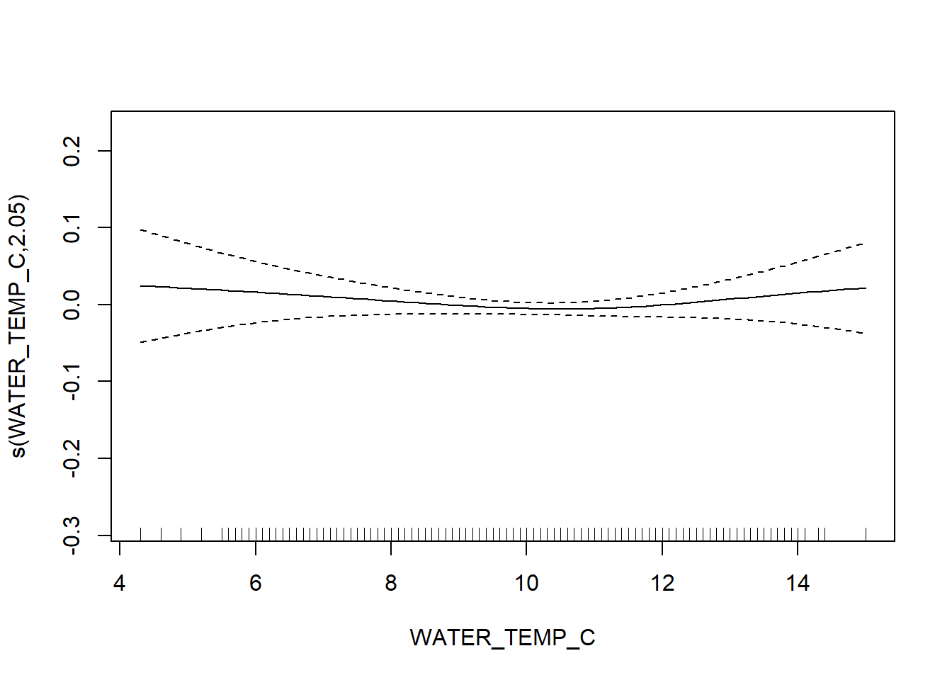
FVCOM data
delta_plus_Fall_FV <- gamm4(delta_plus ~ s(FV_bot_temp) + s(FV_surf_temp) + s(FV_bot_sal) +  s(metric_tons) + s(FV_surf_sal) +  s(START_DEPTH) + s(START_LATITUDE, START_LONGITUDE), random = ~ (1|YEAR) , data = fall_fvcom)

gam.check(delta_plus_Fall_FV$gam)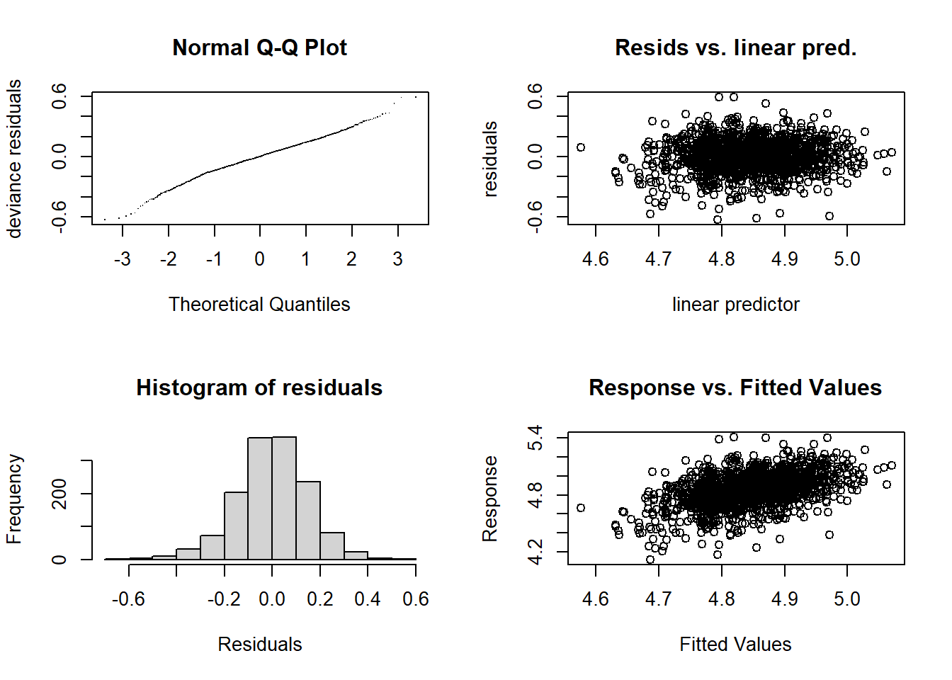
##
## 'gamm' based fit - care required with interpretation.
## Checks based on working residuals may be misleading.
## Basis dimension (k) checking results. Low p-value (k-index<1) may
## indicate that k is too low, especially if edf is close to k'.
##
##                                      k'   edf k-index p-value
## s(FV_bot_temp)                     9.00  1.00    1.00    0.43
## s(FV_surf_temp)                    9.00  3.68    0.96    0.07 .
## s(FV_bot_sal)                      9.00  3.40    0.95    0.04 *
## s(metric_tons)                     9.00  5.60    0.84  <2e-16 ***
## s(FV_surf_sal)                     9.00  4.75    1.00    0.54
## s(START_DEPTH)                     9.00  5.57    1.02    0.81
## s(START_LATITUDE,START_LONGITUDE) 29.00 11.17    0.98    0.17
## ---
## Signif. codes: 0 '***' 0.001 '**' 0.01 '*' 0.05 '.' 0.1 ' ' 1summary(delta_plus_Fall_FV$gam)##
## Family: gaussian
## Link function: identity
##
## Formula:
## delta_plus ~ s(FV_bot_temp) + s(FV_surf_temp) + s(FV_bot_sal) +
## s(metric_tons) + s(FV_surf_sal) + s(START_DEPTH) + s(START_LATITUDE,
## START_LONGITUDE)
##
## Parametric coefficients:
## Estimate Std. Error t value Pr(>|t|)
## (Intercept) 4.844550 0.008326 581.9 <2e-16 ***
## ---
## Signif. codes: 0 '***' 0.001 '**' 0.01 '*' 0.05 '.' 0.1 ' ' 1
##
## Approximate significance of smooth terms:
## edf Ref.df F p-value
## s(FV_bot_temp) 1.000 1.000 0.451 0.502054
## s(FV_surf_temp) 3.677 3.677 2.429 0.111413
## s(FV_bot_sal) 3.397 3.397 1.775 0.133467
## s(metric_tons) 5.604 5.604 4.103 0.000785 ***
## s(FV_surf_sal) 4.748 4.748 4.583 0.000368 ***
## s(START_DEPTH) 5.569 5.569 8.243 < 2e-16 ***
## s(START_LATITUDE,START_LONGITUDE) 11.173 11.173 6.513 < 2e-16 ***
## ---
## Signif. codes: 0 '***' 0.001 '**' 0.01 '*' 0.05 '.' 0.1 ' ' 1
##
## R-sq.(adj) = 0.202
## lmer.REML = -1138.8 Scale est. = 0.023605 n = 1417plot(delta_plus_Fall_FV$gam)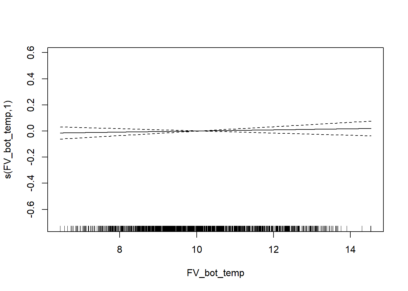
Variation in taxonomic distinctness
survey environmental data
delta_var_Fall <- gamm4(delta_var ~ s(WATER_TEMP_C) + s(SURFACE_TEMP_C) + s(SALINITY) +  s(SURFACE_SALINITY) + s(START_DEPTH)+ s(START_LATITUDE, START_LONGITUDE) +  s(metric_tons), random = ~ (1|YEAR), data = fall)

gam.check(delta_var_Fall$gam)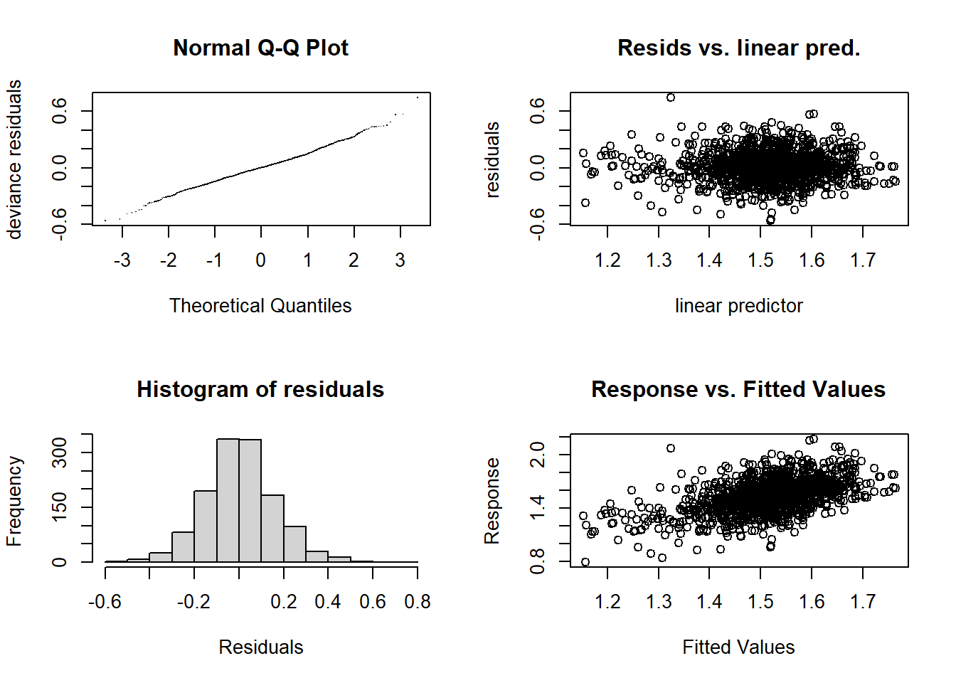
##
## 'gamm' based fit - care required with interpretation.
## Checks based on working residuals may be misleading.
## Basis dimension (k) checking results. Low p-value (k-index<1) may
## indicate that k is too low, especially if edf is close to k'.
##
##                                      k'   edf k-index p-value
## s(WATER_TEMP_C)                    9.00  4.36    0.90  <2e-16 ***
## s(SURFACE_TEMP_C)                  9.00  3.02    0.97    0.10 .
## s(SALINITY)                        9.00  1.00    0.97    0.13
## s(SURFACE_SALINITY)                9.00  1.00    0.96    0.07 .
## s(START_DEPTH)                     9.00  3.72    0.99    0.41
## s(START_LATITUDE,START_LONGITUDE) 29.00 18.96    1.00    0.46
## s(metric_tons)                     9.00  1.99    0.81  <2e-16 ***
## ---
## Signif. codes: 0 '***' 0.001 '**' 0.01 '*' 0.05 '.' 0.1 ' ' 1summary(delta_var_Fall$gam)##
## Family: gaussian
## Link function: identity
##
## Formula:
## delta_var ~ s(WATER_TEMP_C) + s(SURFACE_TEMP_C) + s(SALINITY) +
## s(SURFACE_SALINITY) + s(START_DEPTH) + s(START_LATITUDE,
## START_LONGITUDE) + s(metric_tons)
##
## Parametric coefficients:
## Estimate Std. Error t value Pr(>|t|)
## (Intercept) 1.51453 0.01405 107.8 <2e-16 ***
## ---
## Signif. codes: 0 '***' 0.001 '**' 0.01 '*' 0.05 '.' 0.1 ' ' 1
##
## Approximate significance of smooth terms:
## edf Ref.df F p-value
## s(WATER_TEMP_C) 4.358 4.358 4.694 0.000599 ***
## s(SURFACE_TEMP_C) 3.020 3.020 2.777 0.043585 *
## s(SALINITY) 1.000 1.000 0.382 0.536869
## s(SURFACE_SALINITY) 1.000 1.000 13.413 0.000260 ***
## s(START_DEPTH) 3.722 3.722 7.046 4.07e-05 ***
## s(START_LATITUDE,START_LONGITUDE) 18.961 18.961 9.627 < 2e-16 ***
## s(metric_tons) 1.987 1.987 1.775 0.147340
## ---
## Signif. codes: 0 '***' 0.001 '**' 0.01 '*' 0.05 '.' 0.1 ' ' 1
##
## R-sq.(adj) = 0.242
## lmer.REML = -1032.4 Scale est. = 0.023577 n = 1309plot(delta_var_Fall$gam)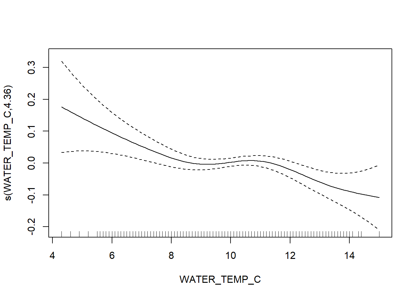
FVCOM data
delta_var_Fall_FV <- gamm4(delta_var ~ s(FV_bot_temp) + s(FV_surf_temp) + s(FV_bot_sal) +  s(metric_tons) +   s(FV_surf_sal) +  s(START_DEPTH) + s(START_LATITUDE, START_LONGITUDE), random = ~ (1|YEAR) , data = fall_fvcom)

gam.check(delta_var_Fall_FV$gam)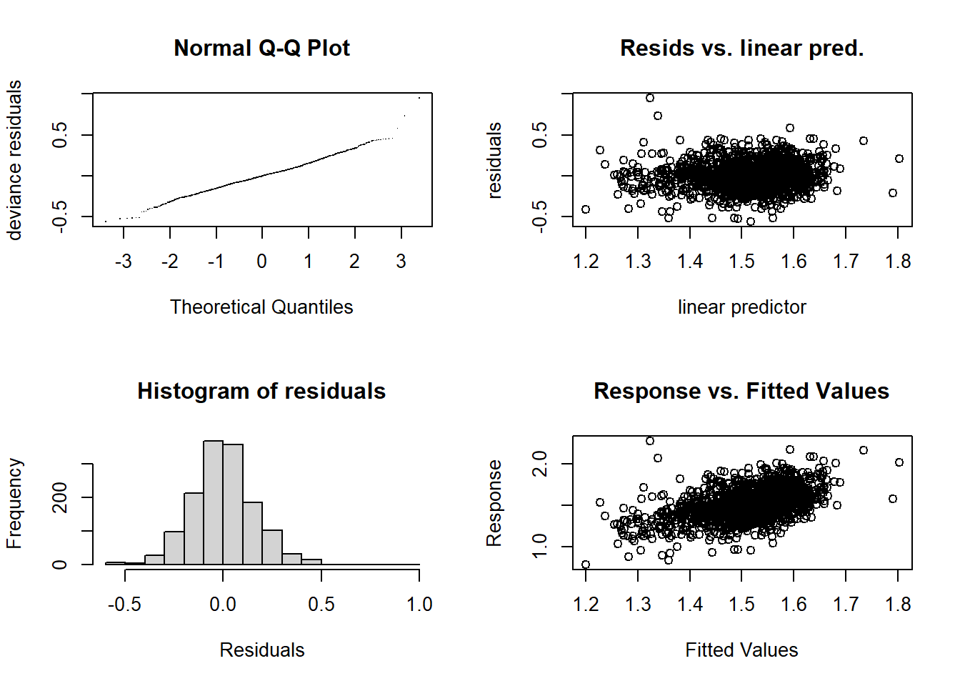
##
## 'gamm' based fit - care required with interpretation.
## Checks based on working residuals may be misleading.
## Basis dimension (k) checking results. Low p-value (k-index<1) may
## indicate that k is too low, especially if edf is close to k'.
##
##                                      k'   edf k-index p-value
## s(FV_bot_temp)                     9.00  2.08    1.01    0.64
## s(FV_surf_temp)                    9.00  1.00    0.96    0.04 *
## s(FV_bot_sal)                      9.00  5.19    1.00    0.42
## s(metric_tons)                     9.00  1.61    0.82  <2e-16 ***
## s(FV_surf_sal)                     9.00  1.00    0.98    0.30
## s(START_DEPTH)                     9.00  2.90    1.01    0.66
## s(START_LATITUDE,START_LONGITUDE) 29.00 18.84    0.99    0.34
## ---
## Signif. codes: 0 '***' 0.001 '**' 0.01 '*' 0.05 '.' 0.1 ' ' 1summary(delta_var_Fall_FV$gam)##
## Family: gaussian
## Link function: identity
##
## Formula:
## delta_var ~ s(FV_bot_temp) + s(FV_surf_temp) + s(FV_bot_sal) +
## s(metric_tons) + s(FV_surf_sal) + s(START_DEPTH) + s(START_LATITUDE,
## START_LONGITUDE)
##
## Parametric coefficients:
## Estimate Std. Error t value Pr(>|t|)
## (Intercept) 1.51418 0.01193 126.9 <2e-16 ***
## ---
## Signif. codes: 0 '***' 0.001 '**' 0.01 '*' 0.05 '.' 0.1 ' ' 1
##
## Approximate significance of smooth terms:
## edf Ref.df F p-value
## s(FV_bot_temp) 2.084 2.084 1.265 0.24971
## s(FV_surf_temp) 1.000 1.000 4.888 0.02721 *
## s(FV_bot_sal) 5.193 5.193 2.465 0.02957 *
## s(metric_tons) 1.612 1.612 0.726 0.32492
## s(FV_surf_sal) 1.000 1.000 6.114 0.01353 *
## s(START_DEPTH) 2.895 2.895 5.720 0.00093 ***
## s(START_LATITUDE,START_LONGITUDE) 18.840 18.840 8.072 < 2e-16 ***
## ---
## Signif. codes: 0 '***' 0.001 '**' 0.01 '*' 0.05 '.' 0.1 ' ' 1
##
## R-sq.(adj) = 0.215
## lmer.REML = -1036.5 Scale est. = 0.025338 n = 1417plot(delta_var_Fall_FV$gam)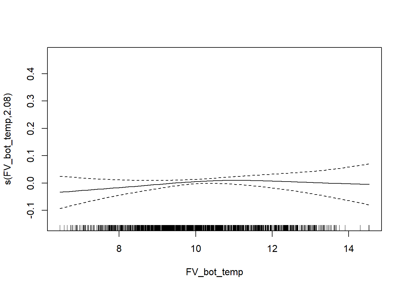
Spring ME-NH GAMMs
- landings data and FVCOM already added to survey data in previous code
# trawl observations
setwd("C:/Users/jjesse/Box/Kerr Lab/Fisheries Science Lab/ME NH Trawl- Seagrant/Seagrant-AEW/Results/GAMMs")

# trawl observations:
spring <- read.csv("ME_NH_spring_exp.csv")

# FVCOM observations
spring_fvcom <- read.csv("ME_NH_spring_full.csv")
Species richness
with survey environmental data
#1 choose response distribution - start w/normal distribution
hist(spring$N_species) # start w/normal distribution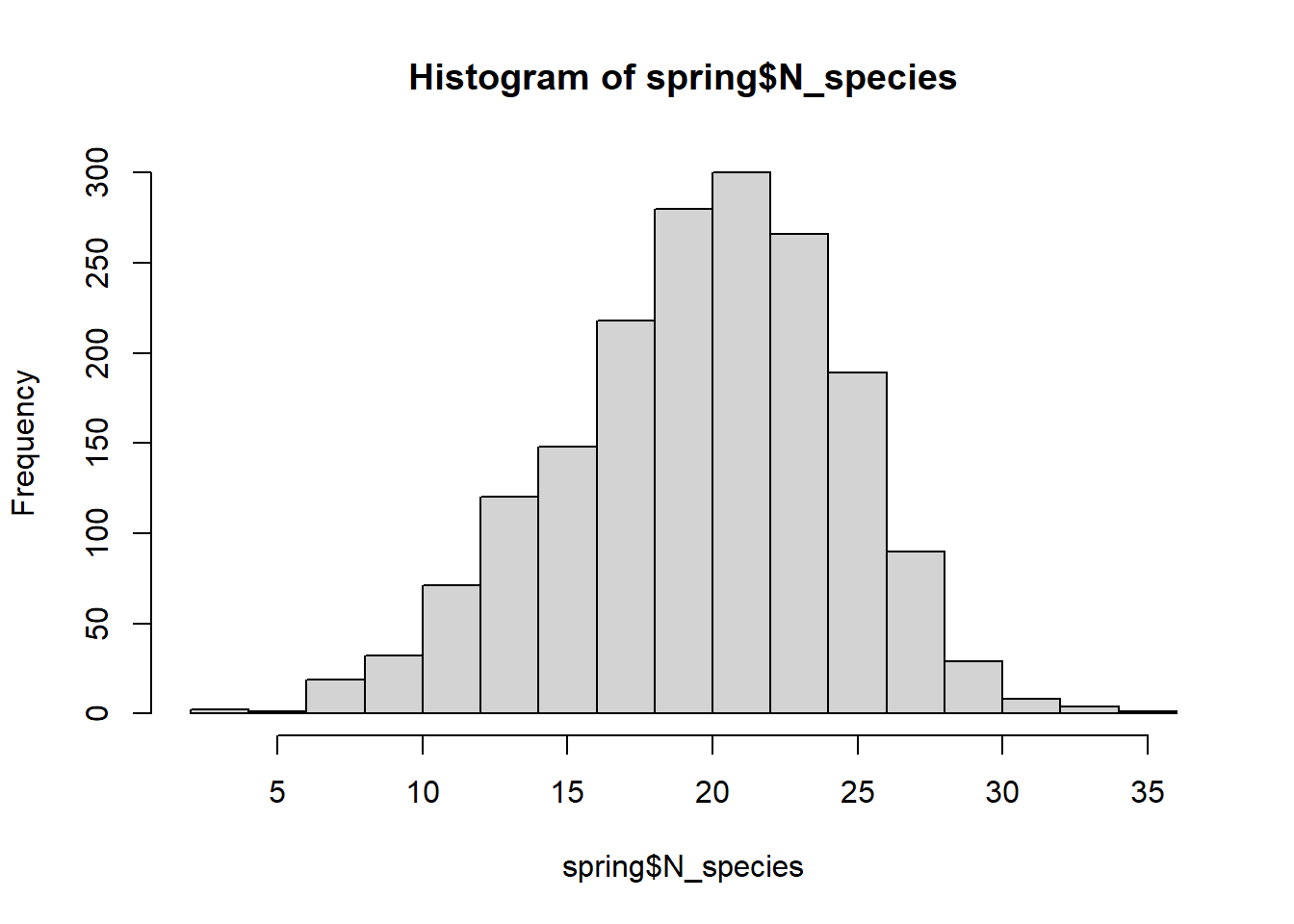
#2 choose k - let GCV find optimal
#3 autocorrelation?
# lat/long = correlated
# bottom/surface salinity = correlated
#plot(spring[,20], spring[,23])
# yes so fit w/GAMM
#4 is k large enough? diagnostics ok?
# diagnostic/residual plots; QQ,resid vs. pred
# take care when interpretting results
# k-index; further below 1 = missed pattern in resids
# k is too low if edf ~ k'
## best model fit is N_Fall_2
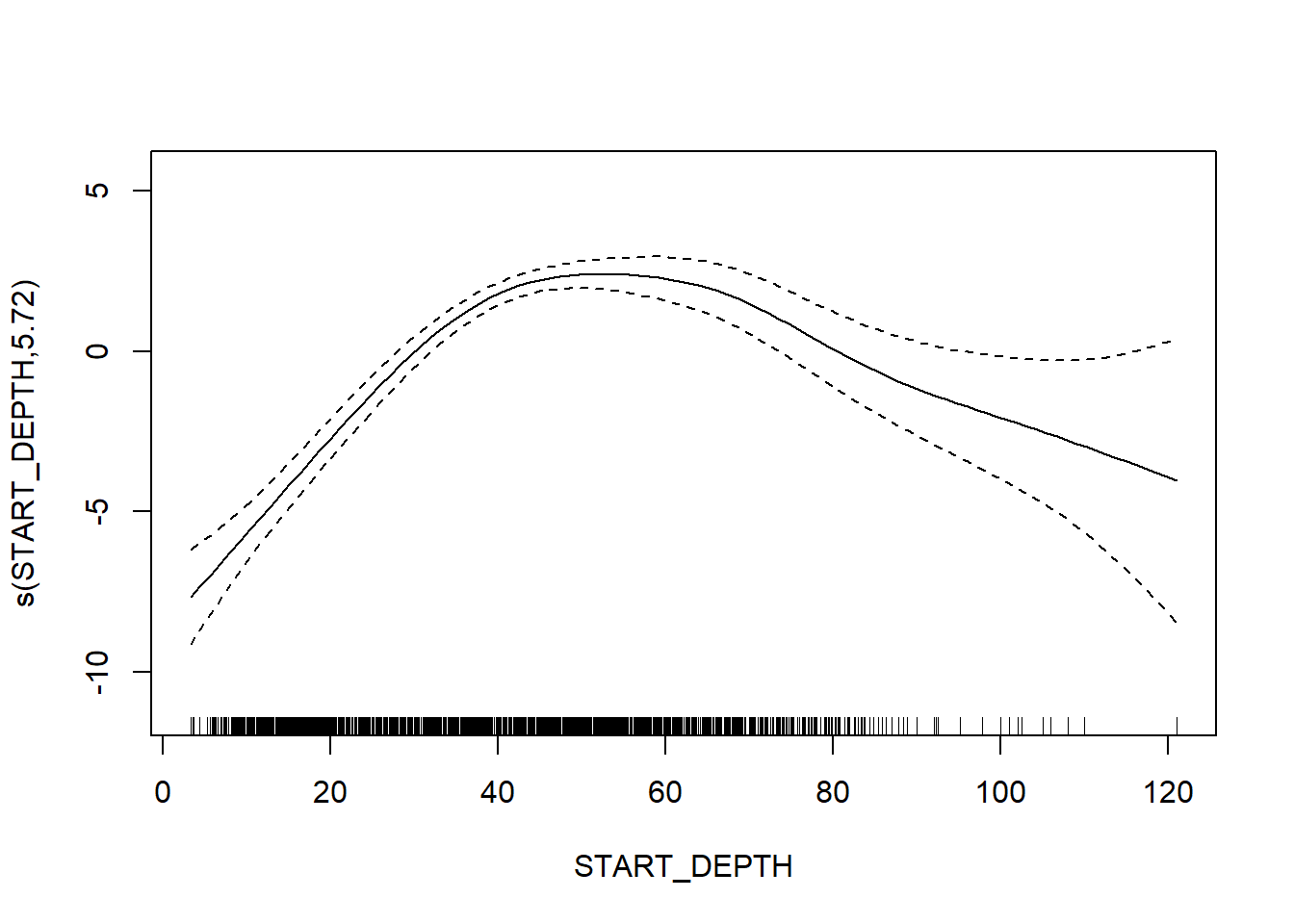
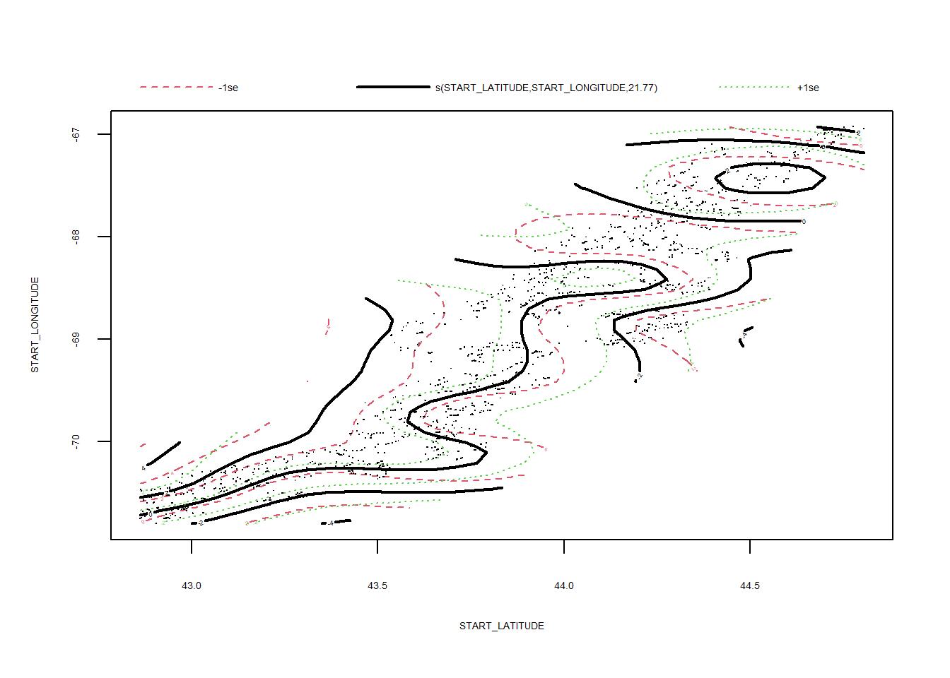
N_spring_2 <- gamm4(N_species ~ s(WATER_TEMP_C) + s(SURFACE_TEMP_C) + s(SALINITY) + s(metric_tons) + s(SURFACE_SALINITY) + s(START_DEPTH) + s(START_LATITUDE, START_LONGITUDE), random = ~ (1|YEAR) , data = spring)
gam.check(N_spring_2$gam)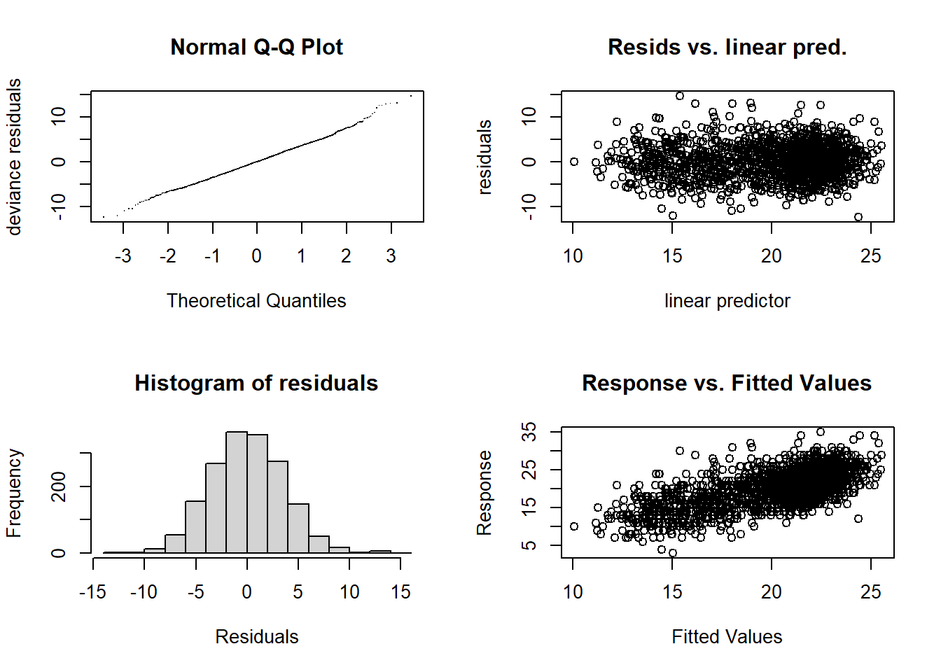
##
## 'gamm' based fit - care required with interpretation.
## Checks based on working residuals may be misleading.
## Basis dimension (k) checking results. Low p-value (k-index<1) may
## indicate that k is too low, especially if edf is close to k'.
##
##                                      k'   edf k-index p-value
## s(WATER_TEMP_C)                    9.00  3.27    0.93  <2e-16 ***
## s(SURFACE_TEMP_C)                  9.00  4.62    0.97   0.135
## s(SALINITY)                        9.00  1.00    0.95   0.005 **
## s(metric_tons)                     9.00  1.53    0.81  <2e-16 ***
## s(SURFACE_SALINITY)                9.00  3.64    1.00   0.425
## s(START_DEPTH)                     9.00  5.72    1.04   0.940
## s(START_LATITUDE,START_LONGITUDE) 29.00 21.77    0.87  <2e-16 ***
## ---
## Signif. codes:  0 '***' 0.001 '**' 0.01 '*' 0.05 '.' 0.1 ' ' 1
#plot(resid(N_spring_2$gam))
#abline(h = 0)
#mean(resid(N_spring_2$gam)^2)
#5 significant trend?
# interpretting results
summary(N_spring_2$gam) # importance of terms ##
## Family: gaussian
## Link function: identity
##
## Formula:
## N_species ~ s(WATER_TEMP_C) + s(SURFACE_TEMP_C) + s(SALINITY) +
## s(metric_tons) + s(SURFACE_SALINITY) + s(START_DEPTH) + s(START_LATITUDE,
## START_LONGITUDE)
##
## Parametric coefficients:
## Estimate Std. Error t value Pr(>|t|)
## (Intercept) 20.0973 0.3014 66.67 <2e-16 ***
## ---
## Signif. codes: 0 '***' 0.001 '**' 0.01 '*' 0.05 '.' 0.1 ' ' 1
##
## Approximate significance of smooth terms:
## edf Ref.df F p-value
## s(WATER_TEMP_C) 3.269 3.269 3.264 0.0218 *
## s(SURFACE_TEMP_C) 4.624 4.624 1.303 0.3629
## s(SALINITY) 1.000 1.000 0.823 0.3645
## s(metric_tons) 1.535 1.535 2.633 0.1725
## s(SURFACE_SALINITY) 3.645 3.645 1.481 0.2123
## s(START_DEPTH) 5.717 5.717 57.366 <2e-16 ***
## s(START_LATITUDE,START_LONGITUDE) 21.772 21.772 6.469 <2e-16 ***
## ---
## Signif. codes: 0 '***' 0.001 '**' 0.01 '*' 0.05 '.' 0.1 ' ' 1
##
## R-sq.(adj) = 0.423
## lmer.REML = 9289.1 Scale est. = 12.243 n = 1714print(N_spring_2$gam) # edf; higher = more complex splines ##
## Family: gaussian
## Link function: identity
##
## Formula:
## N_species ~ s(WATER_TEMP_C) + s(SURFACE_TEMP_C) + s(SALINITY) +
## s(metric_tons) + s(SURFACE_SALINITY) + s(START_DEPTH) + s(START_LATITUDE,
## START_LONGITUDE)
##
## Estimated degrees of freedom:
## 3.27 4.62 1.00 1.53 3.64 5.72 21.77
## total = 42.56
##
## lmer.REML score: 9289.119#confint(N_spring_2$gam)
plot(N_spring_2$gam)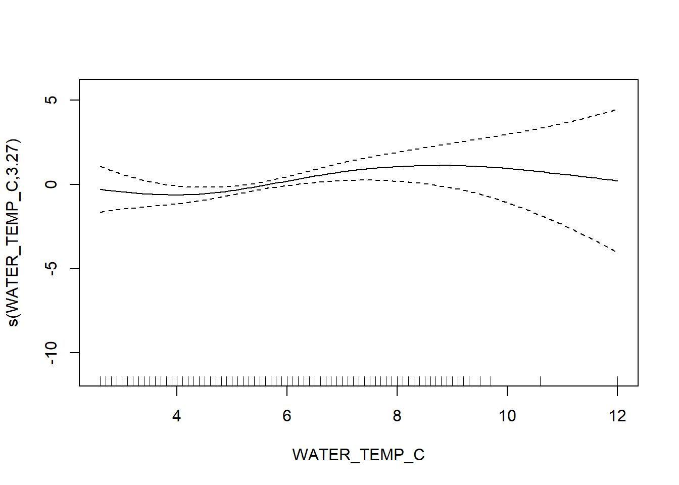
with FVCOM data
N_spring_FV <- gamm4(N_species ~ s(FV_bot_temp) + s(FV_surf_temp) + s(FV_bot_sal) +  s(metric_tons) + s(FV_surf_sal) +  s(START_DEPTH) + s(START_LATITUDE, START_LONGITUDE), random = ~ (1|YEAR) , data = spring_fvcom)

gam.check(N_spring_FV$gam)
##
## 'gamm' based fit - care required with interpretation.
## Checks based on working residuals may be misleading.
## Basis dimension (k) checking results. Low p-value (k-index<1) may
## indicate that k is too low, especially if edf is close to k'.
##
##                                      k'   edf k-index p-value
## s(FV_bot_temp)                     9.00  1.00    1.01   0.590
## s(FV_surf_temp)                    9.00  4.73    0.94   0.005 **
## s(FV_bot_sal)                      9.00  1.00    0.96   0.080 .
## s(metric_tons)                     9.00  1.00    0.77  <2e-16 ***
## s(FV_surf_sal)                     9.00  2.15    0.95   0.030 *
## s(START_DEPTH)                     9.00  5.73    1.02   0.850
## s(START_LATITUDE,START_LONGITUDE) 29.00 20.54    0.89  <2e-16 ***
## ---
## Signif. codes: 0 '***' 0.001 '**' 0.01 '*' 0.05 '.' 0.1 ' ' 1summary(N_spring_FV$gam)##
## Family: gaussian
## Link function: identity
##
## Formula:
## N_species ~ s(FV_bot_temp) + s(FV_surf_temp) + s(FV_bot_sal) +
## s(metric_tons) + s(FV_surf_sal) + s(START_DEPTH) + s(START_LATITUDE,
## START_LONGITUDE)
##
## Parametric coefficients:
## Estimate Std. Error t value Pr(>|t|)
## (Intercept) 20.078 0.346 58.03 <2e-16 ***
## ---
## Signif. codes: 0 '***' 0.001 '**' 0.01 '*' 0.05 '.' 0.1 ' ' 1
##
## Approximate significance of smooth terms:
## edf Ref.df F p-value
## s(FV_bot_temp) 1.000 1.000 0.321 0.57082
## s(FV_surf_temp) 4.727 4.727 5.578 6.34e-05 ***
## s(FV_bot_sal) 1.000 1.000 10.176 0.00145 **
## s(metric_tons) 1.000 1.000 2.104 0.14707
## s(FV_surf_sal) 2.146 2.146 5.331 0.00423 **
## s(START_DEPTH) 5.732 5.732 61.473 < 2e-16 ***
## s(START_LATITUDE,START_LONGITUDE) 20.536 20.536 5.393 < 2e-16 ***
## ---
## Signif. codes: 0 '***' 0.001 '**' 0.01 '*' 0.05 '.' 0.1 ' ' 1
##
## R-sq.(adj) = 0.405
## lmer.REML = 9606.1 Scale est. = 12.149 n = 1778plot(resid(N_spring_FV$gam))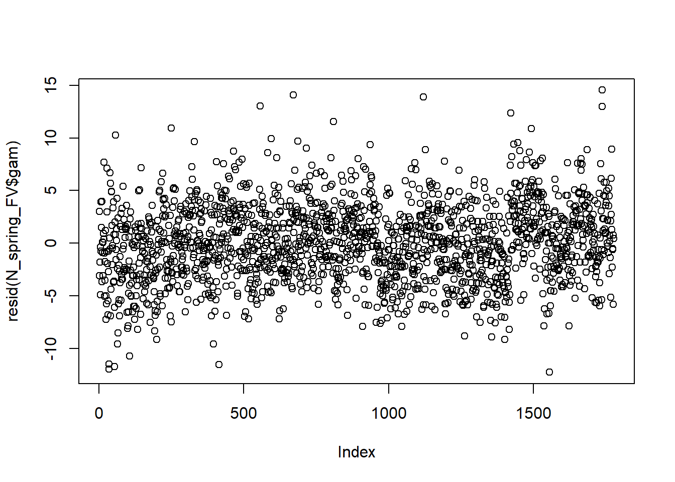
plot(N_spring_FV$gam)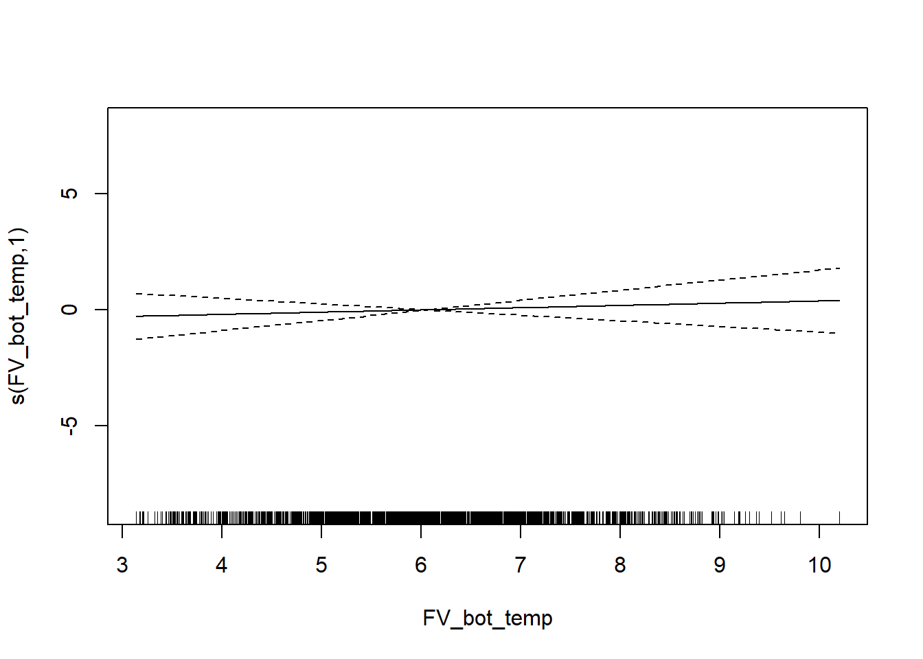
Shannon-Weiner Diversity
survey environmental data
H_spring <-  gamm4(H_index ~ s(WATER_TEMP_C) + s(SURFACE_TEMP_C) + s(SALINITY) + s(SURFACE_SALINITY) + s(START_DEPTH)+ s(START_LATITUDE, START_LONGITUDE) + s(metric_tons), random = ~ (1|YEAR), data = spring)

gam.check(H_spring$gam)
##
## 'gamm' based fit - care required with interpretation.
## Checks based on working residuals may be misleading.
## Basis dimension (k) checking results. Low p-value (k-index<1) may
## indicate that k is too low, especially if edf is close to k'.
##
##                                      k'   edf k-index p-value
## s(WATER_TEMP_C)                    9.00  1.00    0.92  <2e-16 ***
## s(SURFACE_TEMP_C)                  9.00  1.00    0.93  <2e-16 ***
## s(SALINITY)                        9.00  1.00    1.00    0.41
## s(SURFACE_SALINITY)                9.00  3.60    1.00    0.44
## s(START_DEPTH)                     9.00  6.39    1.00    0.50
## s(START_LATITUDE,START_LONGITUDE) 29.00 21.54    0.92  <2e-16 ***
## s(metric_tons)                     9.00  1.26    0.81  <2e-16 ***
## ---
## Signif. codes: 0 '***' 0.001 '**' 0.01 '*' 0.05 '.' 0.1 ' ' 1summary(H_spring$gam)##
## Family: gaussian
## Link function: identity
##
## Formula:
## H_index ~ s(WATER_TEMP_C) + s(SURFACE_TEMP_C) + s(SALINITY) +
## s(SURFACE_SALINITY) + s(START_DEPTH) + s(START_LATITUDE,
## START_LONGITUDE) + s(metric_tons)
##
## Parametric coefficients:
## Estimate Std. Error t value Pr(>|t|)
## (Intercept) 1.26580 0.02894 43.75 <2e-16 ***
## ---
## Signif. codes: 0 '***' 0.001 '**' 0.01 '*' 0.05 '.' 0.1 ' ' 1
##
## Approximate significance of smooth terms:
## edf Ref.df F p-value
## s(WATER_TEMP_C) 1.000 1.000 0.002 0.9638
## s(SURFACE_TEMP_C) 1.000 1.000 0.041 0.8402
## s(SALINITY) 1.000 1.000 6.529 0.0107 *
## s(SURFACE_SALINITY) 3.600 3.600 1.394 0.2603
## s(START_DEPTH) 6.387 6.387 20.685 <2e-16 ***
## s(START_LATITUDE,START_LONGITUDE) 21.544 21.544 16.407 <2e-16 ***
## s(metric_tons) 1.259 1.259 1.344 0.1901
## ---
## Signif. codes: 0 '***' 0.001 '**' 0.01 '*' 0.05 '.' 0.1 ' ' 1
##
## R-sq.(adj) = 0.266
## lmer.REML = 2169.2 Scale est. = 0.1901 n = 1714plot(H_spring$gam)
FVCOM data
H_spring_FV <- gamm4(H_index ~ s(FV_bot_temp) + s(FV_surf_temp) + s(FV_bot_sal) +  s(metric_tons) + s(FV_surf_sal) +  s(START_DEPTH) + s(START_LATITUDE, START_LONGITUDE), random = ~ (1|YEAR) , data = spring_fvcom)

gam.check(H_spring_FV$gam)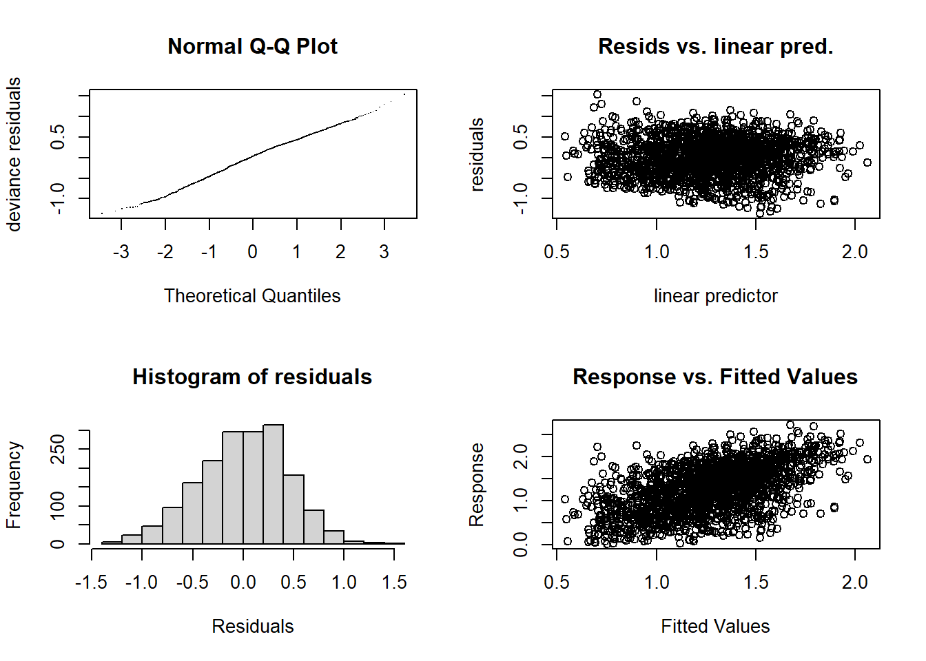
##
## 'gamm' based fit - care required with interpretation.
## Checks based on working residuals may be misleading.
## Basis dimension (k) checking results. Low p-value (k-index<1) may
## indicate that k is too low, especially if edf is close to k'.
##
##                                      k'   edf k-index p-value
## s(FV_bot_temp)                     9.00  1.00    1.00   0.500
## s(FV_surf_temp)                    9.00  4.72    0.97   0.050 *
## s(FV_bot_sal)                      9.00  2.71    0.96   0.035 *
## s(metric_tons)                     9.00  1.00    0.81  <2e-16 ***
## s(FV_surf_sal)                     9.00  2.39    0.99   0.310
## s(START_DEPTH)                     9.00  6.53    1.01   0.585
## s(START_LATITUDE,START_LONGITUDE) 29.00 20.83    0.93  <2e-16 ***
## ---
## Signif. codes: 0 '***' 0.001 '**' 0.01 '*' 0.05 '.' 0.1 ' ' 1summary(H_spring_FV$gam)##
## Family: gaussian
## Link function: identity
##
## Formula:
## H_index ~ s(FV_bot_temp) + s(FV_surf_temp) + s(FV_bot_sal) +
## s(metric_tons) + s(FV_surf_sal) + s(START_DEPTH) + s(START_LATITUDE,
## START_LONGITUDE)
##
## Parametric coefficients:
## Estimate Std. Error t value Pr(>|t|)
## (Intercept) 1.27227 0.03024 42.08 <2e-16 ***
## ---
## Signif. codes: 0 '***' 0.001 '**' 0.01 '*' 0.05 '.' 0.1 ' ' 1
##
## Approximate significance of smooth terms:
## edf Ref.df F p-value
## s(FV_bot_temp) 1.000 1.000 3.500 0.0615 .
## s(FV_surf_temp) 4.716 4.716 2.543 0.0224 *
## s(FV_bot_sal) 2.711 2.711 2.300 0.0903 .
## s(metric_tons) 1.000 1.000 3.288 0.0700 .
## s(FV_surf_sal) 2.391 2.391 0.696 0.5701
## s(START_DEPTH) 6.528 6.528 22.762 <2e-16 ***
## s(START_LATITUDE,START_LONGITUDE) 20.831 20.831 14.629 <2e-16 ***
## ---
## Signif. codes: 0 '***' 0.001 '**' 0.01 '*' 0.05 '.' 0.1 ' ' 1
##
## R-sq.(adj) = 0.27
## lmer.REML = 2241.9 Scale est. = 0.18926 n = 1778plot(H_spring_FV$gam)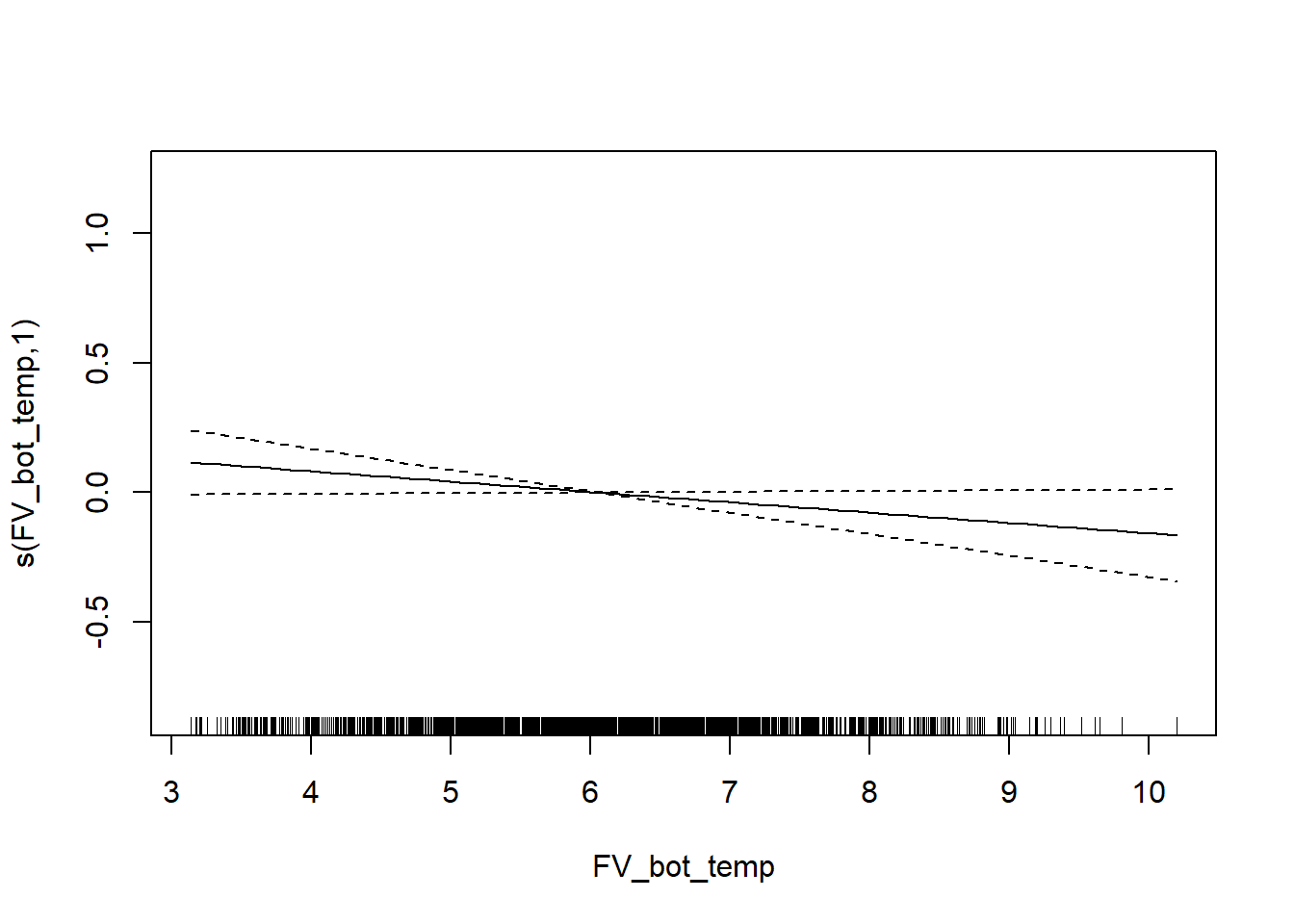
Simpson’s Diversity
survey environmental data
D_spring <- gamm4(D_index  ~ s(WATER_TEMP_C) + s(SURFACE_TEMP_C) + s(SALINITY) + s(SURFACE_SALINITY)  + s(START_DEPTH)+ s(START_LATITUDE, START_LONGITUDE) + s(metric_tons), random = ~ (1|YEAR), data = spring)

gam.check(D_spring$gam)
##
## 'gamm' based fit - care required with interpretation.
## Checks based on working residuals may be misleading.
## Basis dimension (k) checking results. Low p-value (k-index<1) may
## indicate that k is too low, especially if edf is close to k'.
##
##                                      k'   edf k-index p-value
## s(WATER_TEMP_C)                    9.00  1.91    0.95   0.010 **
## s(SURFACE_TEMP_C)                  9.00  1.00    0.95   0.035 *
## s(SALINITY)                        9.00  1.00    1.00   0.620
## s(SURFACE_SALINITY)                9.00  1.00    1.01   0.745
## s(START_DEPTH)                     9.00  6.37    1.01   0.575
## s(START_LATITUDE,START_LONGITUDE) 29.00 20.92    0.92  <2e-16 ***
## s(metric_tons)                     9.00  1.00    0.90  <2e-16 ***
## ---
## Signif. codes: 0 '***' 0.001 '**' 0.01 '*' 0.05 '.' 0.1 ' ' 1summary(D_spring$gam)##
## Family: gaussian
## Link function: identity
##
## Formula:
## D_index ~ s(WATER_TEMP_C) + s(SURFACE_TEMP_C) + s(SALINITY) +
## s(SURFACE_SALINITY) + s(START_DEPTH) + s(START_LATITUDE,
## START_LONGITUDE) + s(metric_tons)
##
## Parametric coefficients:
## Estimate Std. Error t value Pr(>|t|)
## (Intercept) 2.85758 0.06662 42.89 <2e-16 ***
## ---
## Signif. codes: 0 '***' 0.001 '**' 0.01 '*' 0.05 '.' 0.1 ' ' 1
##
## Approximate significance of smooth terms:
## edf Ref.df F p-value
## s(WATER_TEMP_C) 1.914 1.914 0.802 0.4555
## s(SURFACE_TEMP_C) 1.000 1.000 1.302 0.2540
## s(SALINITY) 1.000 1.000 6.492 0.0109 *
## s(SURFACE_SALINITY) 1.000 1.000 0.009 0.9246
## s(START_DEPTH) 6.366 6.366 14.576 <2e-16 ***
## s(START_LATITUDE,START_LONGITUDE) 20.923 20.923 13.783 <2e-16 ***
## s(metric_tons) 1.000 1.000 2.383 0.1228
## ---
## Signif. codes: 0 '***' 0.001 '**' 0.01 '*' 0.05 '.' 0.1 ' ' 1
##
## R-sq.(adj) = 0.212
## lmer.REML = 5918.9 Scale est. = 1.7293 n = 1714plot(D_spring$gam)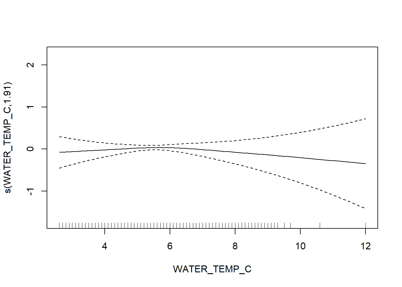
FVCOM data
D_spring_FV <- gamm4(D_index ~ s(FV_bot_temp) + s(FV_surf_temp) + s(FV_bot_sal) +  s(metric_tons) +s(FV_surf_sal) +  s(START_DEPTH) + s(START_LATITUDE, START_LONGITUDE), random = ~ (1|YEAR) , data = spring_fvcom)

gam.check(D_spring_FV$gam)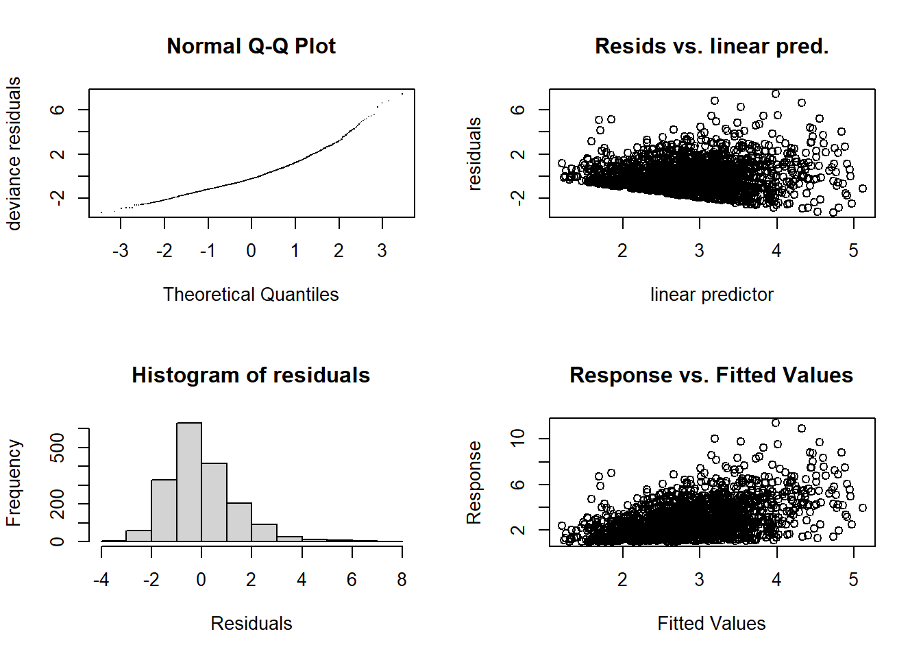
##
## 'gamm' based fit - care required with interpretation.
## Checks based on working residuals may be misleading.
## Basis dimension (k) checking results. Low p-value (k-index<1) may
## indicate that k is too low, especially if edf is close to k'.
##
##                                      k'   edf k-index p-value
## s(FV_bot_temp)                     9.00  1.00    1.01    0.58
## s(FV_surf_temp)                    9.00  3.72    0.98    0.20
## s(FV_bot_sal)                      9.00  1.00    0.98    0.10
## s(metric_tons)                     9.00  1.00    0.89  <2e-16 ***
## s(FV_surf_sal)                     9.00  2.79    1.00    0.49
## s(START_DEPTH)                     9.00  6.41    1.00    0.56
## s(START_LATITUDE,START_LONGITUDE) 29.00 20.44    0.93  <2e-16 ***
## ---
## Signif. codes: 0 '***' 0.001 '**' 0.01 '*' 0.05 '.' 0.1 ' ' 1summary(D_spring_FV$gam)##
## Family: gaussian
## Link function: identity
##
## Formula:
## D_index ~ s(FV_bot_temp) + s(FV_surf_temp) + s(FV_bot_sal) +
## s(metric_tons) + s(FV_surf_sal) + s(START_DEPTH) + s(START_LATITUDE,
## START_LONGITUDE)
##
## Parametric coefficients:
## Estimate Std. Error t value Pr(>|t|)
## (Intercept) 2.88164 0.07446 38.7 <2e-16 ***
## ---
## Signif. codes: 0 '***' 0.001 '**' 0.01 '*' 0.05 '.' 0.1 ' ' 1
##
## Approximate significance of smooth terms:
## edf Ref.df F p-value
## s(FV_bot_temp) 1.000 1.000 3.125 0.0773 .
## s(FV_surf_temp) 3.720 3.720 2.568 0.0245 *
## s(FV_bot_sal) 1.000 1.000 5.451 0.0197 *
## s(metric_tons) 1.000 1.000 3.905 0.0483 *
## s(FV_surf_sal) 2.794 2.794 1.261 0.3295
## s(START_DEPTH) 6.411 6.411 14.688 <2e-16 ***
## s(START_LATITUDE,START_LONGITUDE) 20.435 20.435 12.108 <2e-16 ***
## ---
## Signif. codes: 0 '***' 0.001 '**' 0.01 '*' 0.05 '.' 0.1 ' ' 1
##
## R-sq.(adj) = 0.212
## lmer.REML = 6173.9 Scale est. = 1.7601 n = 1778plot(D_spring_FV$gam)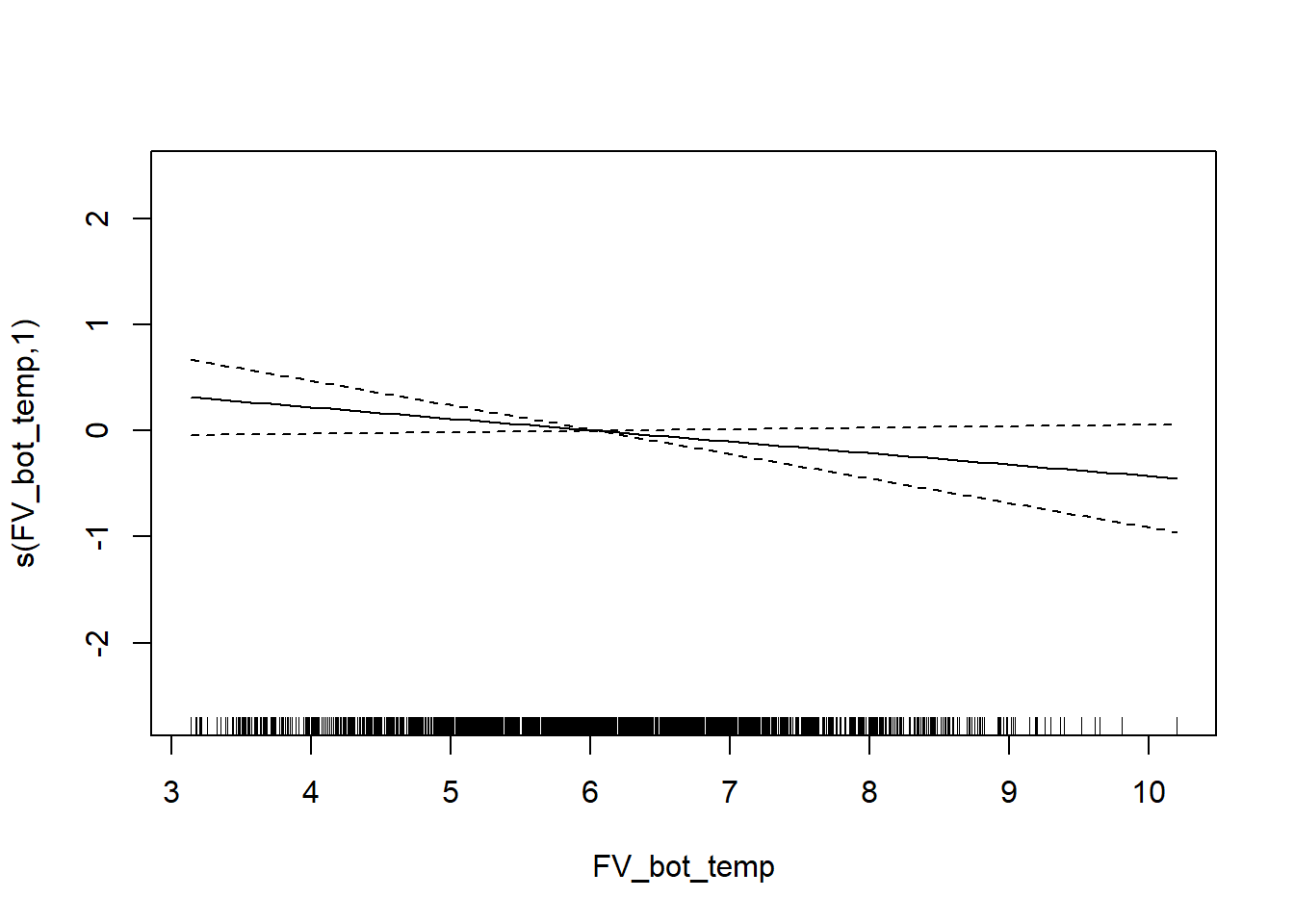

Simpson’s Evenness
survey environmental data
E_spring <- gamm4(E_index  ~ s(WATER_TEMP_C) + s(SURFACE_TEMP_C) + s(SALINITY) +  s(SURFACE_SALINITY) + s(START_DEPTH)+ s(START_LATITUDE, START_LONGITUDE) + s(metric_tons), random = ~ (1|YEAR), data = spring)

gam.check(E_spring$gam)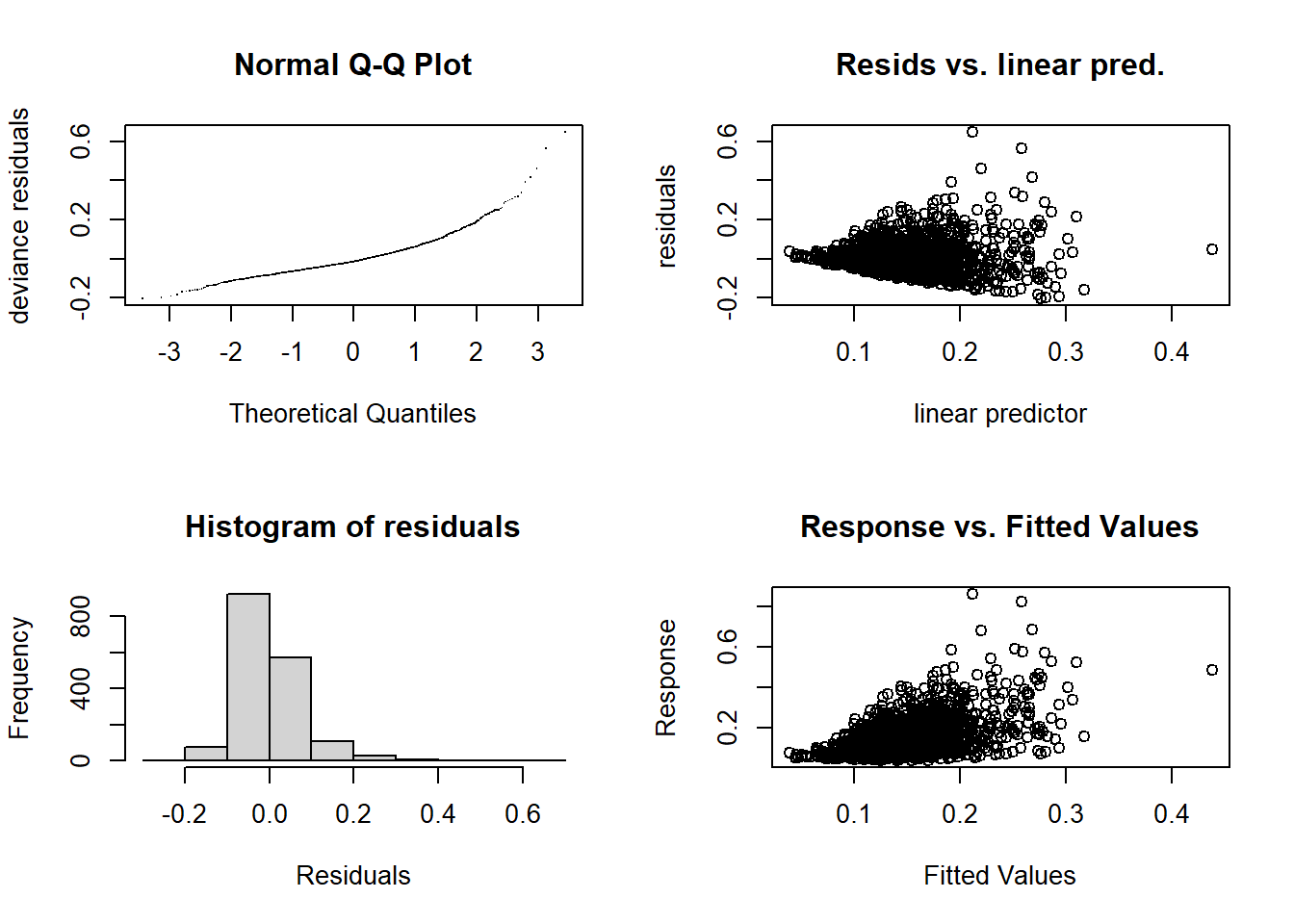
##
## 'gamm' based fit - care required with interpretation.
## Checks based on working residuals may be misleading.
## Basis dimension (k) checking results. Low p-value (k-index<1) may
## indicate that k is too low, especially if edf is close to k'.
##
##                                      k'   edf k-index p-value
## s(WATER_TEMP_C)                    9.00  2.61    0.94   0.005 **
## s(SURFACE_TEMP_C)                  9.00  1.00    0.97   0.095 .
## s(SALINITY)                        9.00  3.24    0.99   0.315
## s(SURFACE_SALINITY)                9.00  3.78    1.04   0.965
## s(START_DEPTH)                     9.00  5.70    1.00   0.495
## s(START_LATITUDE,START_LONGITUDE) 29.00 21.67    0.89  <2e-16 ***
## s(metric_tons)                     9.00  1.00    0.93  <2e-16 ***
## ---
## Signif. codes: 0 '***' 0.001 '**' 0.01 '*' 0.05 '.' 0.1 ' ' 1summary(E_spring$gam)##
## Family: gaussian
## Link function: identity
##
## Formula:
## E_index ~ s(WATER_TEMP_C) + s(SURFACE_TEMP_C) + s(SALINITY) +
## s(SURFACE_SALINITY) + s(START_DEPTH) + s(START_LATITUDE,
## START_LONGITUDE) + s(metric_tons)
##
## Parametric coefficients:
## Estimate Std. Error t value Pr(>|t|)
## (Intercept) 0.149612 0.004007 37.34 <2e-16 ***
## ---
## Signif. codes: 0 '***' 0.001 '**' 0.01 '*' 0.05 '.' 0.1 ' ' 1
##
## Approximate significance of smooth terms:
## edf Ref.df F p-value
## s(WATER_TEMP_C) 2.608 2.608 2.649 0.1101
## s(SURFACE_TEMP_C) 1.000 1.000 1.718 0.1901
## s(SALINITY) 3.239 3.239 2.546 0.0469 *
## s(SURFACE_SALINITY) 3.781 3.781 2.118 0.0476 *
## s(START_DEPTH) 5.700 5.700 6.940 1.03e-06 ***
## s(START_LATITUDE,START_LONGITUDE) 21.666 21.666 10.642 < 2e-16 ***
## s(metric_tons) 1.000 1.000 4.692 0.0304 *
## ---
## Signif. codes: 0 '***' 0.001 '**' 0.01 '*' 0.05 '.' 0.1 ' ' 1
##
## R-sq.(adj) = 0.23
## lmer.REML = -3753.4 Scale est. = 0.0059014 n = 1714plot(E_spring$gam)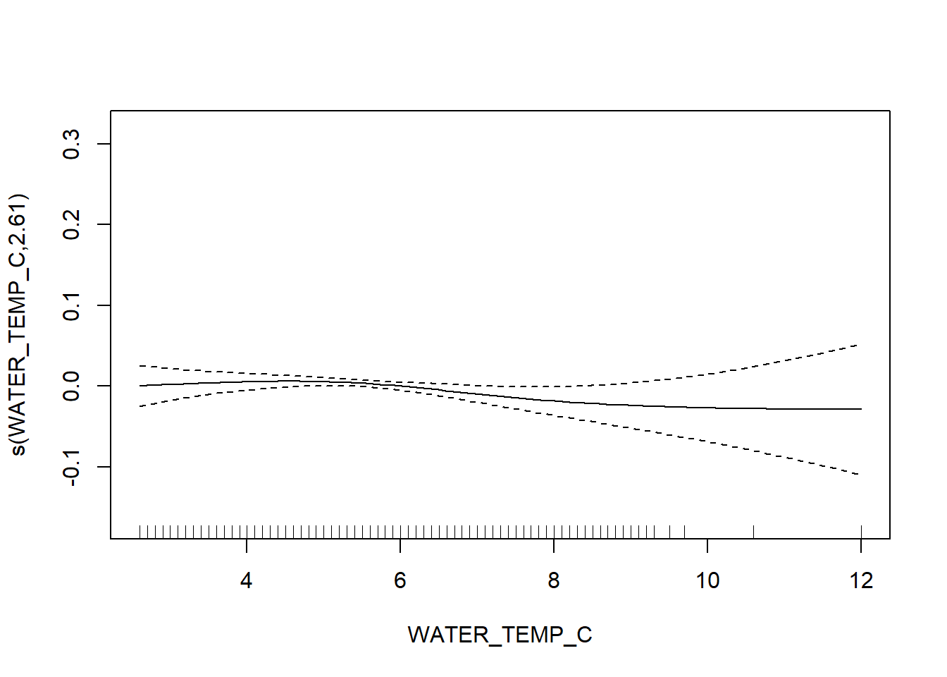
FVCOM data
E_spring_FV <- gamm4(E_index ~ s(FV_bot_temp) + s(FV_surf_temp) + s(FV_bot_sal) +  s(metric_tons) + s(FV_surf_sal) +  s(START_DEPTH) + s(START_LATITUDE, START_LONGITUDE), random = ~ (1|YEAR) , data = spring_fvcom)

gam.check(E_spring_FV$gam)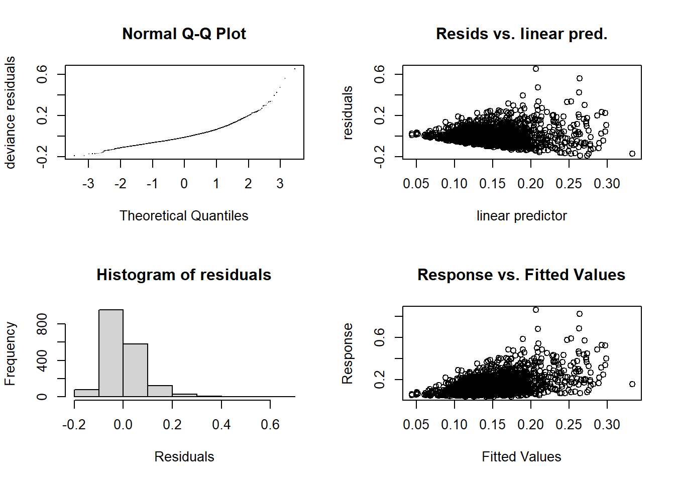
##
## 'gamm' based fit - care required with interpretation.
## Checks based on working residuals may be misleading.
## Basis dimension (k) checking results. Low p-value (k-index<1) may
## indicate that k is too low, especially if edf is close to k'.
##
##                                      k'   edf k-index p-value
## s(FV_bot_temp)                     9.00  1.82    1.01   0.715
## s(FV_surf_temp)                    9.00  1.00    0.97   0.095 .
## s(FV_bot_sal)                      9.00  1.00    0.97   0.120
## s(metric_tons)                     9.00  1.00    0.92  <2e-16 ***
## s(FV_surf_sal)                     9.00  2.82    1.02   0.740
## s(START_DEPTH)                     9.00  5.64    1.00   0.575
## s(START_LATITUDE,START_LONGITUDE) 29.00 21.61    0.89  <2e-16 ***
## ---
## Signif. codes: 0 '***' 0.001 '**' 0.01 '*' 0.05 '.' 0.1 ' ' 1summary(E_spring_FV$gam)##
## Family: gaussian
## Link function: identity
##
## Formula:
## E_index ~ s(FV_bot_temp) + s(FV_surf_temp) + s(FV_bot_sal) +
## s(metric_tons) + s(FV_surf_sal) + s(START_DEPTH) + s(START_LATITUDE,
## START_LONGITUDE)
##
## Parametric coefficients:
## Estimate Std. Error t value Pr(>|t|)
## (Intercept) 0.150668 0.004555 33.08 <2e-16 ***
## ---
## Signif. codes: 0 '***' 0.001 '**' 0.01 '*' 0.05 '.' 0.1 ' ' 1
##
## Approximate significance of smooth terms:
## edf Ref.df F p-value
## s(FV_bot_temp) 1.819 1.819 2.496 0.1653
## s(FV_surf_temp) 1.000 1.000 0.198 0.6562
## s(FV_bot_sal) 1.000 1.000 3.694 0.0548 .
## s(metric_tons) 1.000 1.000 6.249 0.0125 *
## s(FV_surf_sal) 2.816 2.816 0.977 0.3460
## s(START_DEPTH) 5.643 5.643 5.576 1.4e-05 ***
## s(START_LATITUDE,START_LONGITUDE) 21.610 21.610 12.263 < 2e-16 ***
## ---
## Signif. codes: 0 '***' 0.001 '**' 0.01 '*' 0.05 '.' 0.1 ' ' 1
##
## R-sq.(adj) = 0.22
## lmer.REML = -3867.3 Scale est. = 0.006036 n = 1778plot(E_spring_FV$gam)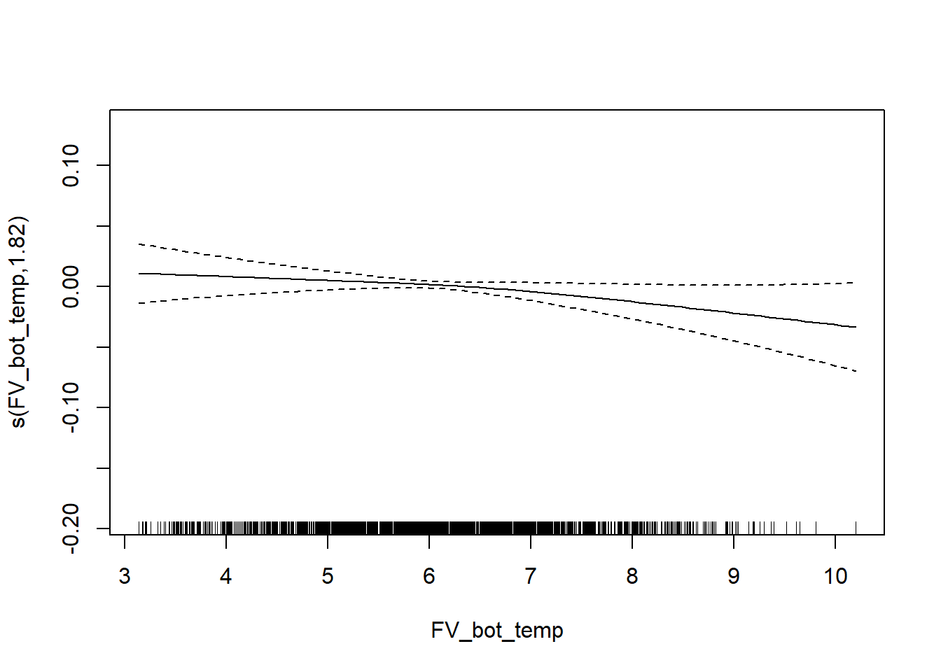

Taxonomic diversity
survey environmental data
delta_spring <- gamm4(delta ~ s(WATER_TEMP_C) + s(SURFACE_TEMP_C) + s(SALINITY) + s(SURFACE_SALINITY) + s(START_DEPTH)+ s(START_LATITUDE, START_LONGITUDE) +  s(metric_tons), random = ~ (1|YEAR), data = spring)

gam.check(delta_spring$gam)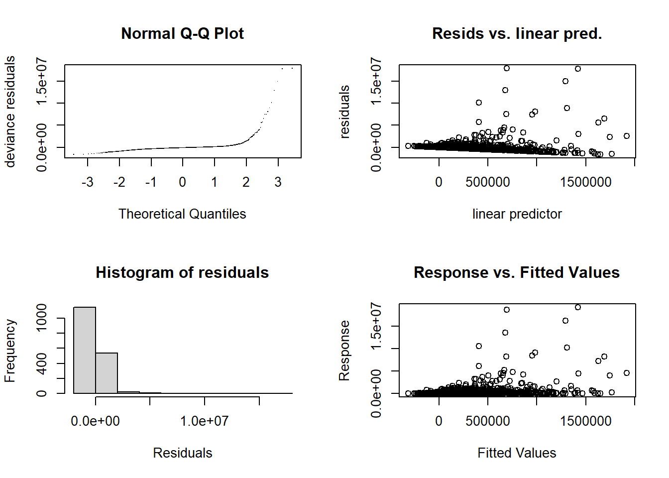
##
## 'gamm' based fit - care required with interpretation.
## Checks based on working residuals may be misleading.
## Basis dimension (k) checking results. Low p-value (k-index<1) may
## indicate that k is too low, especially if edf is close to k'.
##
##                                      k'   edf k-index p-value
## s(WATER_TEMP_C)                    9.00  1.00    1.01   0.650
## s(SURFACE_TEMP_C)                  9.00  1.78    0.97   0.095 .
## s(SALINITY)                        9.00  1.00    1.00   0.495
## s(SURFACE_SALINITY)                9.00  3.78    1.03   0.980
## s(START_DEPTH)                     9.00  4.50    1.01   0.745
## s(START_LATITUDE,START_LONGITUDE) 29.00 15.42    1.00   0.485
## s(metric_tons)                     9.00  1.00    0.86  <2e-16 ***
## ---
## Signif. codes: 0 '***' 0.001 '**' 0.01 '*' 0.05 '.' 0.1 ' ' 1summary(delta_spring$gam)##
## Family: gaussian
## Link function: identity
##
## Formula:
## delta ~ s(WATER_TEMP_C) + s(SURFACE_TEMP_C) + s(SALINITY) + s(SURFACE_SALINITY) +
## s(START_DEPTH) + s(START_LATITUDE, START_LONGITUDE) + s(metric_tons)
##
## Parametric coefficients:
## Estimate Std. Error t value Pr(>|t|)
## (Intercept) 274488 46588 5.892 4.6e-09 ***
## ---
## Signif. codes: 0 '***' 0.001 '**' 0.01 '*' 0.05 '.' 0.1 ' ' 1
##
## Approximate significance of smooth terms:
## edf Ref.df F p-value
## s(WATER_TEMP_C) 1.000 1.000 0.029 0.8654
## s(SURFACE_TEMP_C) 1.783 1.783 4.964 0.0272 *
## s(SALINITY) 1.000 1.000 0.654 0.4189
## s(SURFACE_SALINITY) 3.777 3.777 2.512 0.0422 *
## s(START_DEPTH) 4.498 4.498 1.432 0.1265
## s(START_LATITUDE,START_LONGITUDE) 15.415 15.415 3.883 8.04e-07 ***
## s(metric_tons) 1.000 1.000 3.051 0.0809 .
## ---
## Signif. codes: 0 '***' 0.001 '**' 0.01 '*' 0.05 '.' 0.1 ' ' 1
##
## R-sq.(adj) = 0.0768
## lmer.REML = 52239 Scale est. = 1.1032e+12 n = 1714plot(delta_spring$gam)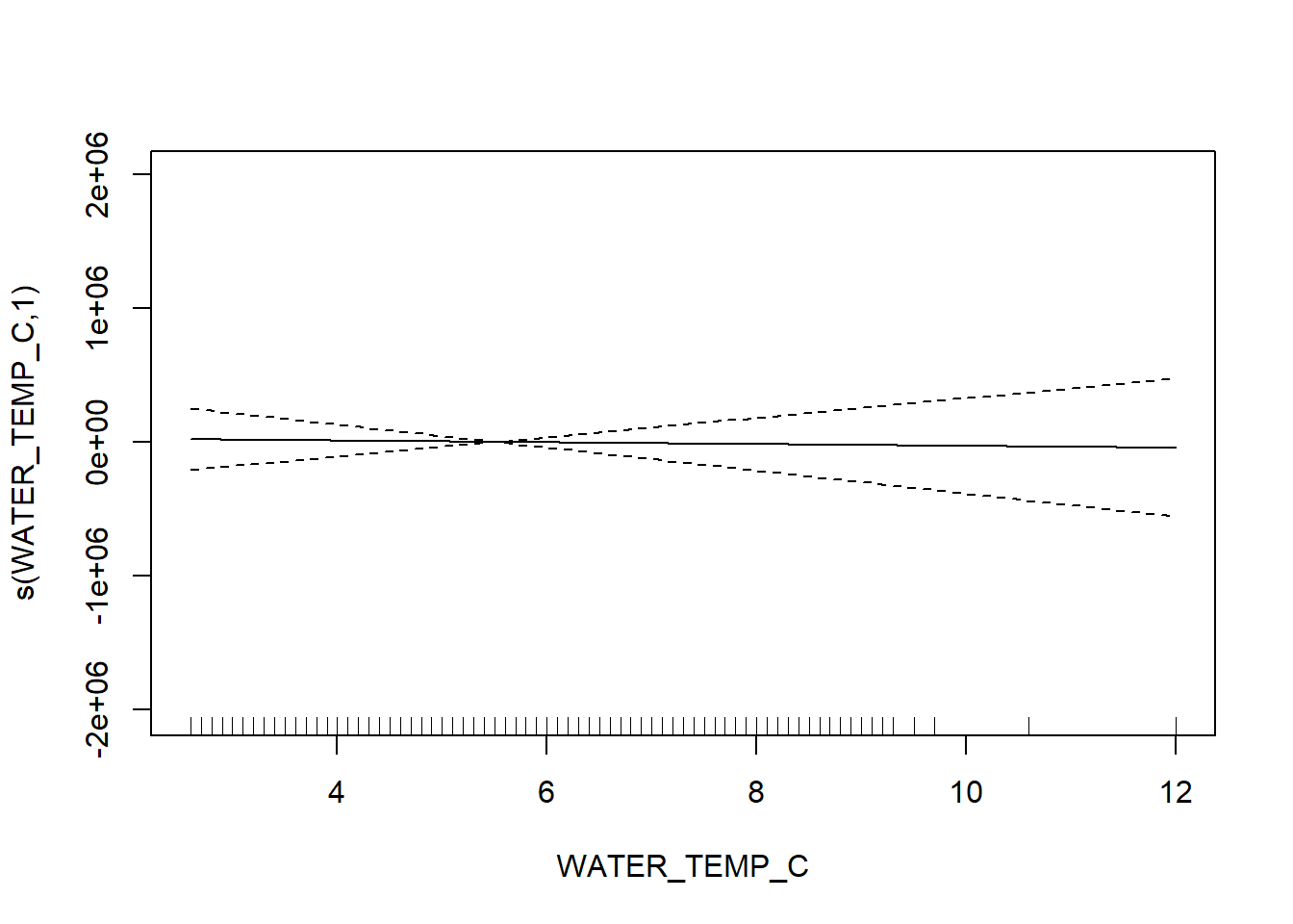


FVCOM data
delta_spring_FV <- gamm4(delta ~ s(FV_bot_temp) + s(FV_surf_temp) + s(FV_bot_sal) +  s(metric_tons) +s(FV_surf_sal) +  s(START_DEPTH) + s(START_LATITUDE, START_LONGITUDE), random = ~ (1|YEAR) , data = spring_fvcom)

gam.check(delta_spring_FV$gam)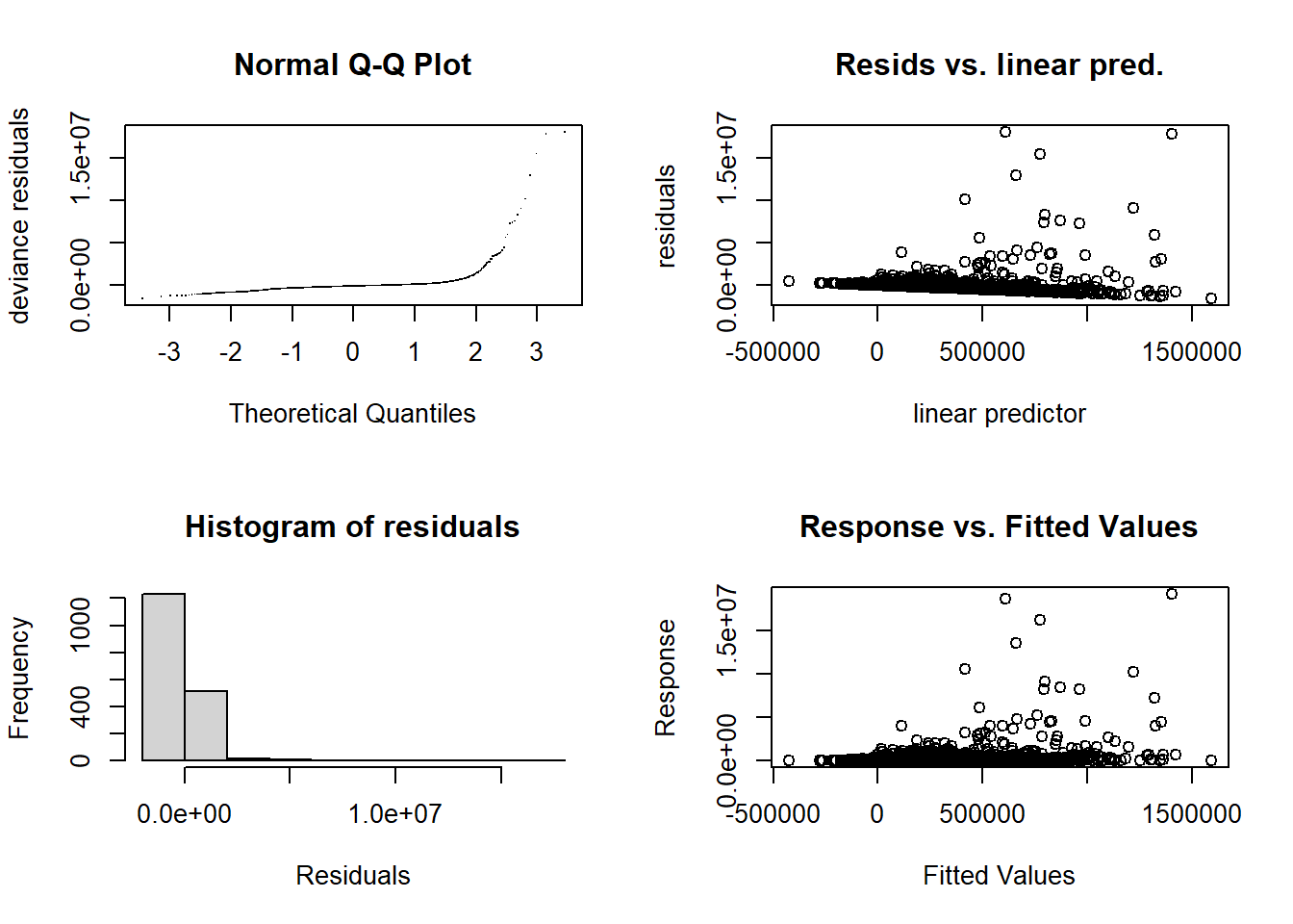
##
## 'gamm' based fit - care required with interpretation.
## Checks based on working residuals may be misleading.
## Basis dimension (k) checking results. Low p-value (k-index<1) may
## indicate that k is too low, especially if edf is close to k'.
##
##                                      k'   edf k-index p-value
## s(FV_bot_temp)                     9.00  1.00    1.00   0.420
## s(FV_surf_temp)                    9.00  1.00    0.98   0.130
## s(FV_bot_sal)                      9.00  1.00    1.02   0.870
## s(metric_tons)                     9.00  1.00    0.85  <2e-16 ***
## s(FV_surf_sal)                     9.00  1.00    0.93   0.005 **
## s(START_DEPTH)                     9.00  5.06    1.01   0.615
## s(START_LATITUDE,START_LONGITUDE) 29.00 16.28    1.01   0.535
## ---
## Signif. codes: 0 '***' 0.001 '**' 0.01 '*' 0.05 '.' 0.1 ' ' 1summary(delta_spring_FV$gam)##
## Family: gaussian
## Link function: identity
##
## Formula:
## delta ~ s(FV_bot_temp) + s(FV_surf_temp) + s(FV_bot_sal) + s(metric_tons) +
## s(FV_surf_sal) + s(START_DEPTH) + s(START_LATITUDE, START_LONGITUDE)
##
## Parametric coefficients:
## Estimate Std. Error t value Pr(>|t|)
## (Intercept) 271220 50286 5.394 7.85e-08 ***
## ---
## Signif. codes: 0 '***' 0.001 '**' 0.01 '*' 0.05 '.' 0.1 ' ' 1
##
## Approximate significance of smooth terms:
## edf Ref.df F p-value
## s(FV_bot_temp) 1.000 1.000 1.300 0.2543
## s(FV_surf_temp) 1.000 1.000 0.561 0.4538
## s(FV_bot_sal) 1.000 1.000 0.337 0.5615
## s(metric_tons) 1.000 1.000 2.354 0.1252
## s(FV_surf_sal) 1.000 1.000 0.007 0.9322
## s(START_DEPTH) 5.056 5.056 2.666 0.0234 *
## s(START_LATITUDE,START_LONGITUDE) 16.283 16.283 3.869 5.78e-07 ***
## ---
## Signif. codes: 0 '***' 0.001 '**' 0.01 '*' 0.05 '.' 0.1 ' ' 1
##
## R-sq.(adj) = 0.0655
## lmer.REML = 54157 Scale est. = 1.0802e+12 n = 1778plot(delta_spring_FV$gam)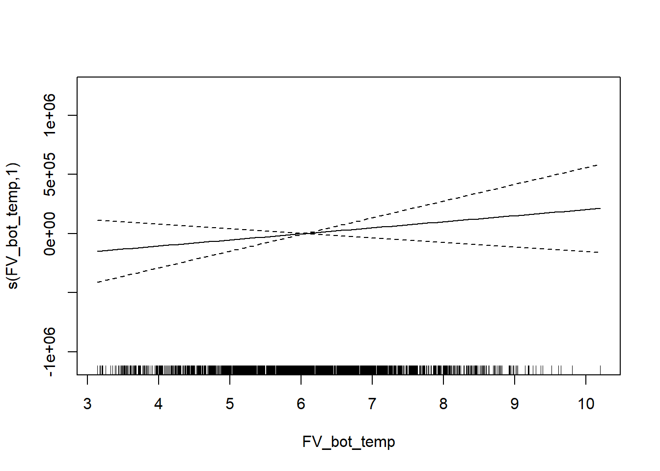

Taxonomic distinctness
survey environmental data
delta_star_spring <- gamm4(delta_star ~ s(WATER_TEMP_C) + s(SURFACE_TEMP_C) + s(SALINITY) +  s(SURFACE_SALINITY) + s(START_DEPTH)+ s(START_LATITUDE, START_LONGITUDE) +  s(metric_tons), random = ~ (1|YEAR), data = spring)

gam.check(delta_star_spring$gam)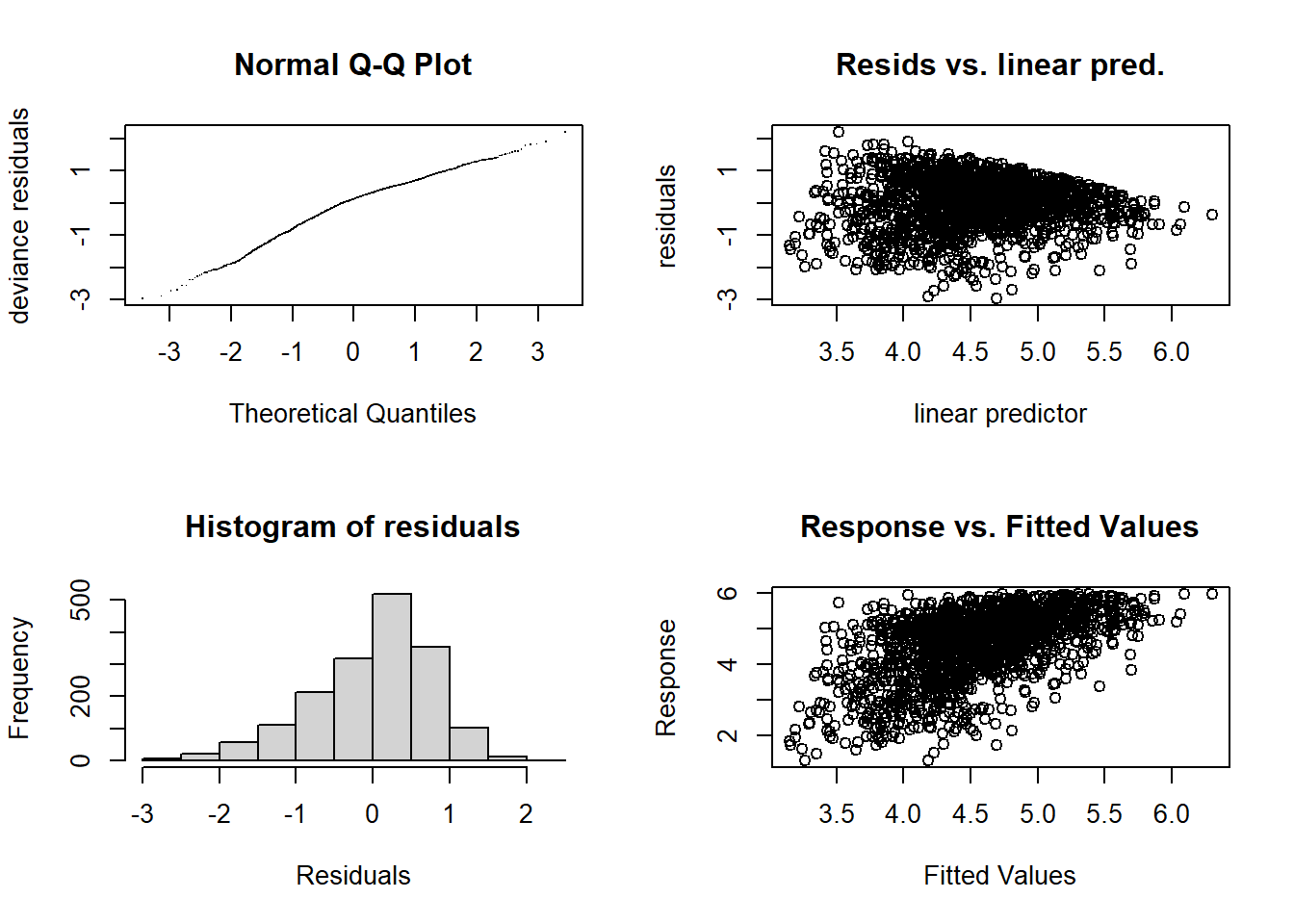
##
## 'gamm' based fit - care required with interpretation.
## Checks based on working residuals may be misleading.
## Basis dimension (k) checking results. Low p-value (k-index<1) may
## indicate that k is too low, especially if edf is close to k'.
##
##                                      k'   edf k-index p-value
## s(WATER_TEMP_C)                    9.00  1.50    0.86  <2e-16 ***
## s(SURFACE_TEMP_C)                  9.00  2.84    0.91  <2e-16 ***
## s(SALINITY)                        9.00  1.00    0.97   0.110
## s(SURFACE_SALINITY)                9.00  4.37    1.00   0.430
## s(START_DEPTH)                     9.00  4.54    1.00   0.450
## s(START_LATITUDE,START_LONGITUDE) 29.00 24.99    0.95   0.005 **
## s(metric_tons)                     9.00  1.00    0.74  <2e-16 ***
## ---
## Signif. codes: 0 '***' 0.001 '**' 0.01 '*' 0.05 '.' 0.1 ' ' 1summary(delta_star_spring$gam)##
## Family: gaussian
## Link function: identity
##
## Formula:
## delta_star ~ s(WATER_TEMP_C) + s(SURFACE_TEMP_C) + s(SALINITY) +
## s(SURFACE_SALINITY) + s(START_DEPTH) + s(START_LATITUDE,
## START_LONGITUDE) + s(metric_tons)
##
## Parametric coefficients:
## Estimate Std. Error t value Pr(>|t|)
## (Intercept) 4.55632 0.04726 96.4 <2e-16 ***
## ---
## Signif. codes: 0 '***' 0.001 '**' 0.01 '*' 0.05 '.' 0.1 ' ' 1
##
## Approximate significance of smooth terms:
## edf Ref.df F p-value
## s(WATER_TEMP_C) 1.495 1.495 0.188 0.774567
## s(SURFACE_TEMP_C) 2.839 2.839 2.414 0.050721 .
## s(SALINITY) 1.000 1.000 1.578 0.209180
## s(SURFACE_SALINITY) 4.374 4.374 3.713 0.005063 **
## s(START_DEPTH) 4.537 4.537 29.639 < 2e-16 ***
## s(START_LATITUDE,START_LONGITUDE) 24.991 24.991 18.055 < 2e-16 ***
## s(metric_tons) 1.000 1.000 14.371 0.000156 ***
## ---
## Signif. codes: 0 '***' 0.001 '**' 0.01 '*' 0.05 '.' 0.1 ' ' 1
##
## R-sq.(adj) = 0.292
## lmer.REML = 4137.2 Scale est. = 0.59711 n = 1714plot(delta_star_spring$gam)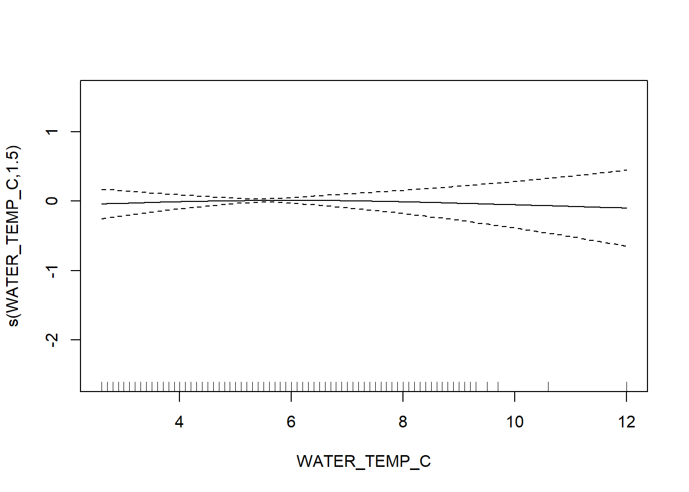

FVCOM data
delta_star_spring_FV <- gamm4(delta_star ~ s(FV_bot_temp) + s(FV_surf_temp) + s(FV_bot_sal) +  s(metric_tons) + s(FV_surf_sal) +  s(START_DEPTH) + s(START_LATITUDE, START_LONGITUDE), random = ~ (1|YEAR) , data = spring_fvcom)

gam.check(delta_star_spring_FV$gam)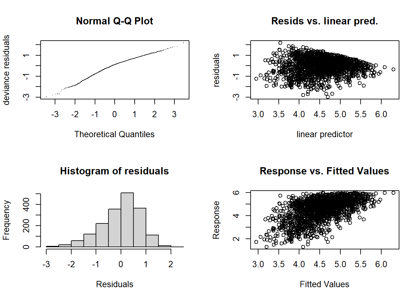
##
## 'gamm' based fit - care required with interpretation.
## Checks based on working residuals may be misleading.
## Basis dimension (k) checking results. Low p-value (k-index<1) may
## indicate that k is too low, especially if edf is close to k'.
##
##                                      k'   edf k-index p-value
## s(FV_bot_temp)                     9.00  1.00    0.95   0.010 **
## s(FV_surf_temp)                    9.00  1.00    0.94   0.005 **
## s(FV_bot_sal)                      9.00  6.86    0.97   0.120
## s(metric_tons)                     9.00  1.00    0.75  <2e-16 ***
## s(FV_surf_sal)                     9.00  1.00    0.96   0.045 *
## s(START_DEPTH)                     9.00  4.64    1.01   0.550
## s(START_LATITUDE,START_LONGITUDE) 29.00 24.76    0.95   0.010 **
## ---
## Signif. codes: 0 '***' 0.001 '**' 0.01 '*' 0.05 '.' 0.1 ' ' 1summary(delta_star_spring_FV$gam)##
## Family: gaussian
## Link function: identity
##
## Formula:
## delta_star ~ s(FV_bot_temp) + s(FV_surf_temp) + s(FV_bot_sal) +
## s(metric_tons) + s(FV_surf_sal) + s(START_DEPTH) + s(START_LATITUDE,
## START_LONGITUDE)
##
## Parametric coefficients:
## Estimate Std. Error t value Pr(>|t|)
## (Intercept) 4.55844 0.05293 86.11 <2e-16 ***
## ---
## Signif. codes: 0 '***' 0.001 '**' 0.01 '*' 0.05 '.' 0.1 ' ' 1
##
## Approximate significance of smooth terms:
## edf Ref.df F p-value
## s(FV_bot_temp) 1.000 1.000 6.620 0.01016 *
## s(FV_surf_temp) 1.000 1.000 6.671 0.00988 **
## s(FV_bot_sal) 6.859 6.859 5.680 1.24e-06 ***
## s(metric_tons) 1.000 1.000 11.982 0.00055 ***
## s(FV_surf_sal) 1.000 1.000 2.351 0.12539
## s(START_DEPTH) 4.642 4.642 31.689 < 2e-16 ***
## s(START_LATITUDE,START_LONGITUDE) 24.762 24.762 17.829 < 2e-16 ***
## ---
## Signif. codes: 0 '***' 0.001 '**' 0.01 '*' 0.05 '.' 0.1 ' ' 1
##
## R-sq.(adj) = 0.292
## lmer.REML = 4245.3 Scale est. = 0.58191 n = 1778plot(delta_star_spring_FV$gam)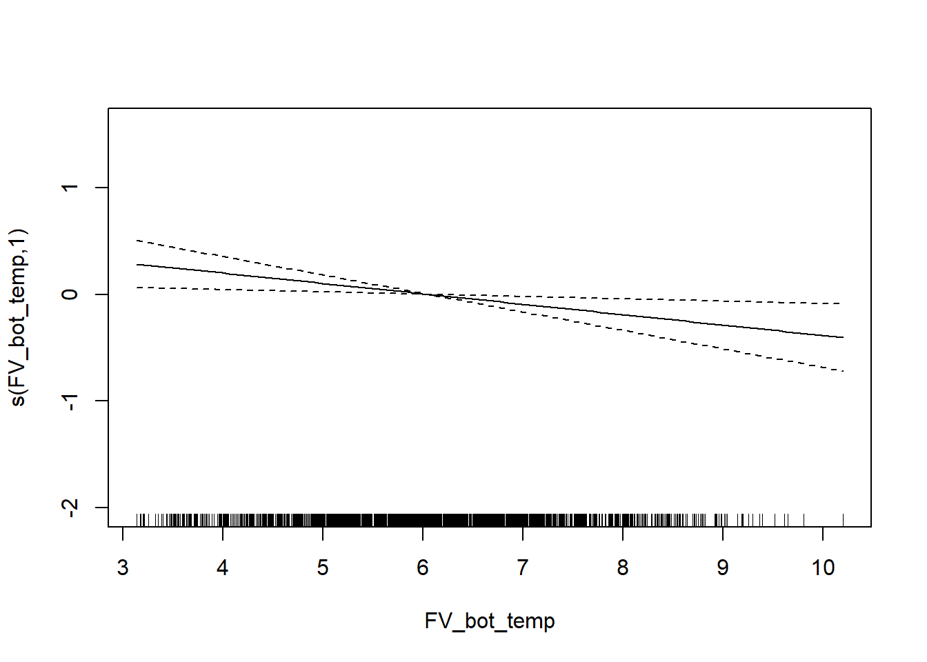

Average taxonomic distinctness
survey environmental data
delta_plus_spring <- gamm4(delta_plus ~ s(WATER_TEMP_C) + s(SURFACE_TEMP_C) + s(SALINITY) +  s(SURFACE_SALINITY) + s(START_DEPTH)+ s(START_LATITUDE, START_LONGITUDE) +  s(metric_tons), random = ~ (1|YEAR), data = spring_fvcom)

gam.check(delta_plus_spring$gam)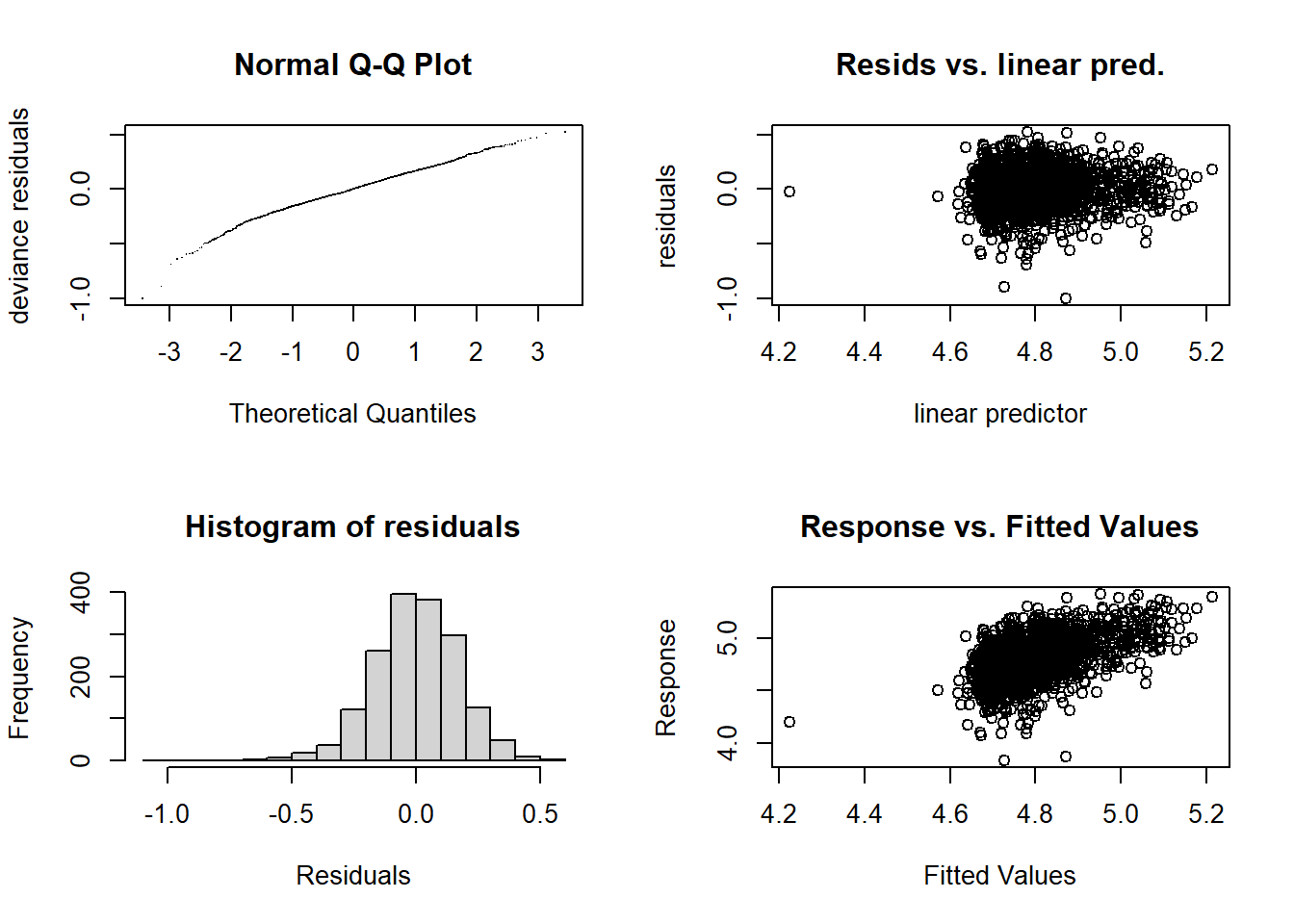
##
## 'gamm' based fit - care required with interpretation.
## Checks based on working residuals may be misleading.
## Basis dimension (k) checking results. Low p-value (k-index<1) may
## indicate that k is too low, especially if edf is close to k'.
##
##                                      k'   edf k-index p-value
## s(WATER_TEMP_C)                    9.00  1.63    0.98   0.230
## s(SURFACE_TEMP_C)                  9.00  3.19    1.00   0.490
## s(SALINITY)                        9.00  1.00    0.98   0.155
## s(SURFACE_SALINITY)                9.00  2.16    0.97   0.105
## s(START_DEPTH)                     9.00  4.88    0.94   0.015 *
## s(START_LATITUDE,START_LONGITUDE) 29.00 23.30    0.93  <2e-16 ***
## s(metric_tons)                     9.00  1.99    0.90  <2e-16 ***
## ---
## Signif. codes: 0 '***' 0.001 '**' 0.01 '*' 0.05 '.' 0.1 ' ' 1summary(delta_plus_spring$gam)##
## Family: gaussian
## Link function: identity
##
## Formula:
## delta_plus ~ s(WATER_TEMP_C) + s(SURFACE_TEMP_C) + s(SALINITY) +
## s(SURFACE_SALINITY) + s(START_DEPTH) + s(START_LATITUDE,
## START_LONGITUDE) + s(metric_tons)
##
## Parametric coefficients:
## Estimate Std. Error t value Pr(>|t|)
## (Intercept) 4.80129 0.00856 560.9 <2e-16 ***
## ---
## Signif. codes: 0 '***' 0.001 '**' 0.01 '*' 0.05 '.' 0.1 ' ' 1
##
## Approximate significance of smooth terms:
## edf Ref.df F p-value
## s(WATER_TEMP_C) 1.631 1.631 0.471 0.45217
## s(SURFACE_TEMP_C) 3.187 3.187 3.416 0.01530 *
## s(SALINITY) 1.000 1.000 0.098 0.75398
## s(SURFACE_SALINITY) 2.162 2.162 6.215 0.00197 **
## s(START_DEPTH) 4.883 4.883 15.152 < 2e-16 ***
## s(START_LATITUDE,START_LONGITUDE) 23.298 23.298 10.020 < 2e-16 ***
## s(metric_tons) 1.988 1.988 2.539 0.09552 .
## ---
## Signif. codes: 0 '***' 0.001 '**' 0.01 '*' 0.05 '.' 0.1 ' ' 1
##
## R-sq.(adj) = 0.247
## lmer.REML = -976.84 Scale est. = 0.030083 n = 1714plot(delta_plus_spring$gam)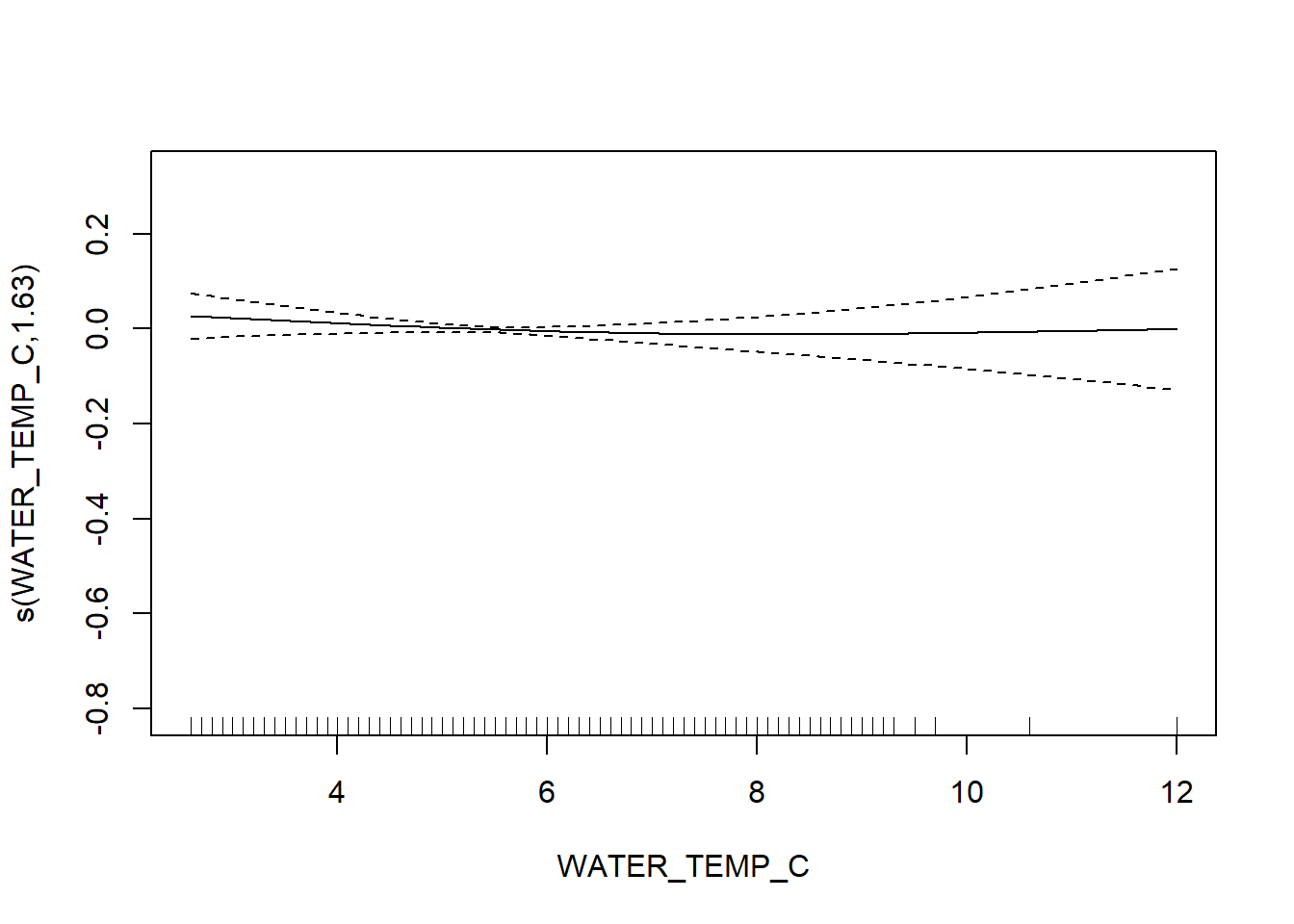
FVCOM data
delta_plus_spring_FV <- gamm4(delta_plus ~ s(FV_bot_temp) + s(FV_surf_temp) + s(FV_bot_sal) +  s(metric_tons) + s(FV_surf_sal) +  s(START_DEPTH) + s(START_LATITUDE, START_LONGITUDE), random = ~ (1|YEAR) , data = spring_fvcom)

gam.check(delta_plus_spring_FV$gam)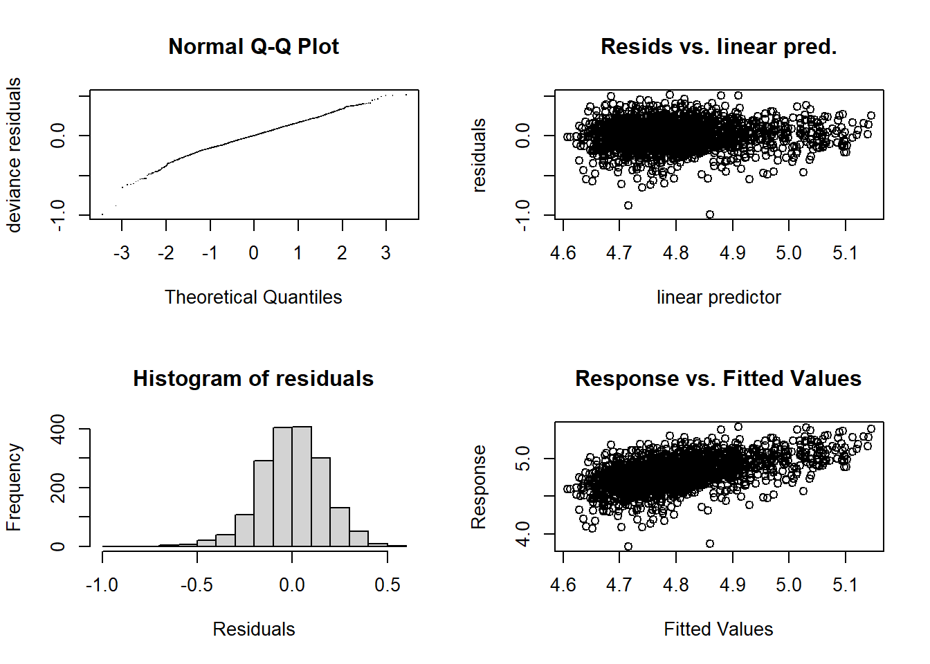
##
## 'gamm' based fit - care required with interpretation.
## Checks based on working residuals may be misleading.
## Basis dimension (k) checking results. Low p-value (k-index<1) may
## indicate that k is too low, especially if edf is close to k'.
##
##                                      k'   edf k-index p-value
## s(FV_bot_temp)                     9.00  3.12    1.01    0.67
## s(FV_surf_temp)                    9.00  3.89    0.99    0.34
## s(FV_bot_sal)                      9.00  4.20    0.98    0.23
## s(metric_tons)                     9.00  1.89    0.90  <2e-16 ***
## s(FV_surf_sal)                     9.00  1.29    1.00    0.58
## s(START_DEPTH)                     9.00  5.00    0.96    0.05 *
## s(START_LATITUDE,START_LONGITUDE) 29.00 23.85    0.93  <2e-16 ***
## ---
## Signif. codes: 0 '***' 0.001 '**' 0.01 '*' 0.05 '.' 0.1 ' ' 1summary(delta_plus_spring_FV$gam)##
## Family: gaussian
## Link function: identity
##
## Formula:
## delta_plus ~ s(FV_bot_temp) + s(FV_surf_temp) + s(FV_bot_sal) +
## s(metric_tons) + s(FV_surf_sal) + s(START_DEPTH) + s(START_LATITUDE,
## START_LONGITUDE)
##
## Parametric coefficients:
## Estimate Std. Error t value Pr(>|t|)
## (Intercept) 4.802616 0.009383 511.9 <2e-16 ***
## ---
## Signif. codes: 0 '***' 0.001 '**' 0.01 '*' 0.05 '.' 0.1 ' ' 1
##
## Approximate significance of smooth terms:
## edf Ref.df F p-value
## s(FV_bot_temp) 3.122 3.122 2.815 0.0315 *
## s(FV_surf_temp) 3.886 3.886 2.284 0.0382 *
## s(FV_bot_sal) 4.200 4.200 2.834 0.0273 *
## s(metric_tons) 1.891 1.891 1.810 0.2357
## s(FV_surf_sal) 1.290 1.290 4.362 0.0228 *
## s(START_DEPTH) 5.001 5.001 14.365 <2e-16 ***
## s(START_LATITUDE,START_LONGITUDE) 23.849 23.849 10.066 <2e-16 ***
## ---
## Signif. codes: 0 '***' 0.001 '**' 0.01 '*' 0.05 '.' 0.1 ' ' 1
##
## R-sq.(adj) = 0.251
## lmer.REML = -1034.5 Scale est. = 0.02958 n = 1778plot(delta_plus_spring_FV$gam)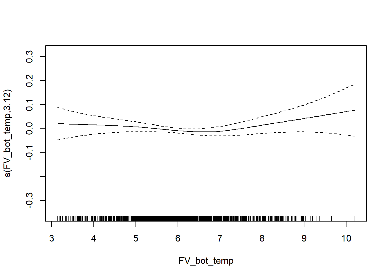
Variation in taxonomic distinctness
survey environmental data
delta_var_spring <- gamm4(delta_var ~ s(WATER_TEMP_C) + s(SURFACE_TEMP_C) + s(SALINITY) +  s(SURFACE_SALINITY) + s(START_DEPTH)+ s(START_LATITUDE, START_LONGITUDE) +  s(metric_tons), random = ~ (1|YEAR), data = spring)

gam.check(delta_var_spring$gam)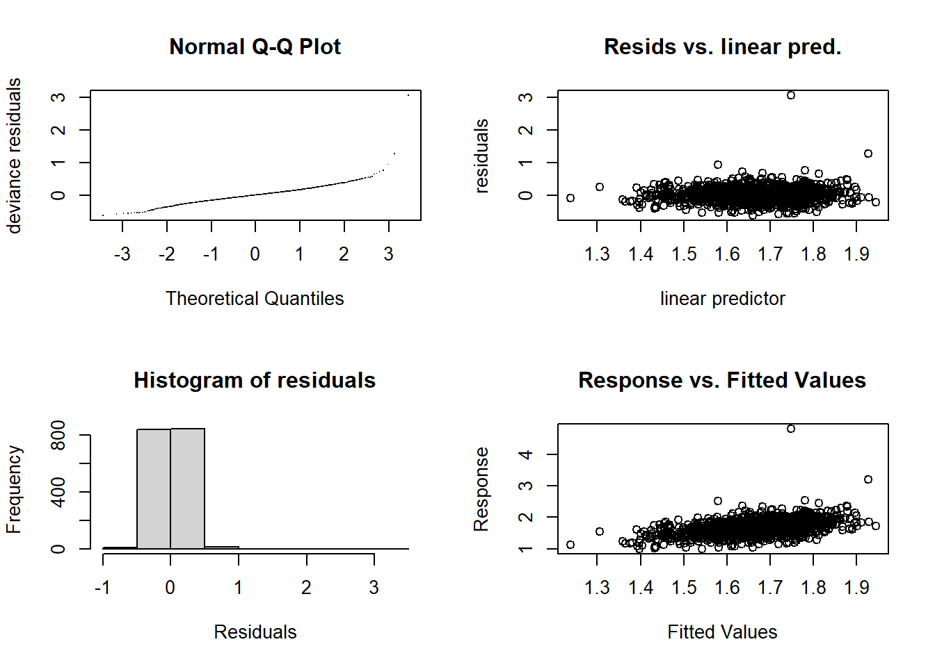
##
## 'gamm' based fit - care required with interpretation.
## Checks based on working residuals may be misleading.
## Basis dimension (k) checking results. Low p-value (k-index<1) may
## indicate that k is too low, especially if edf is close to k'.
##
##                                      k'   edf k-index p-value
## s(WATER_TEMP_C)                    9.00  3.20    0.96   0.060 .
## s(SURFACE_TEMP_C)                  9.00  3.80    1.00   0.495
## s(SALINITY)                        9.00  2.45    1.00   0.405
## s(SURFACE_SALINITY)                9.00  1.00    0.98   0.115
## s(START_DEPTH)                     9.00  4.32    0.93   0.005 **
## s(START_LATITUDE,START_LONGITUDE) 29.00 15.52    1.00   0.515
## s(metric_tons)                     9.00  1.00    0.94   0.005 **
## ---
## Signif. codes: 0 '***' 0.001 '**' 0.01 '*' 0.05 '.' 0.1 ' ' 1summary(delta_var_spring$gam)##
## Family: gaussian
## Link function: identity
##
## Formula:
## delta_var ~ s(WATER_TEMP_C) + s(SURFACE_TEMP_C) + s(SALINITY) +
## s(SURFACE_SALINITY) + s(START_DEPTH) + s(START_LATITUDE,
## START_LONGITUDE) + s(metric_tons)
##
## Parametric coefficients:
## Estimate Std. Error t value Pr(>|t|)
## (Intercept) 1.68364 0.01143 147.4 <2e-16 ***
## ---
## Signif. codes: 0 '***' 0.001 '**' 0.01 '*' 0.05 '.' 0.1 ' ' 1
##
## Approximate significance of smooth terms:
## edf Ref.df F p-value
## s(WATER_TEMP_C) 3.196 3.196 4.277 0.00562 **
## s(SURFACE_TEMP_C) 3.797 3.797 4.842 0.00143 **
## s(SALINITY) 2.451 2.451 2.365 0.11043
## s(SURFACE_SALINITY) 1.000 1.000 2.425 0.11964
## s(START_DEPTH) 4.315 4.315 10.427 < 2e-16 ***
## s(START_LATITUDE,START_LONGITUDE) 15.523 15.523 14.803 < 2e-16 ***
## s(metric_tons) 1.000 1.000 1.892 0.16919
## ---
## Signif. codes: 0 '***' 0.001 '**' 0.01 '*' 0.05 '.' 0.1 ' ' 1
##
## R-sq.(adj) = 0.196
## lmer.REML = -614.44 Scale est. = 0.037737 n = 1714plot(delta_var_spring$gam)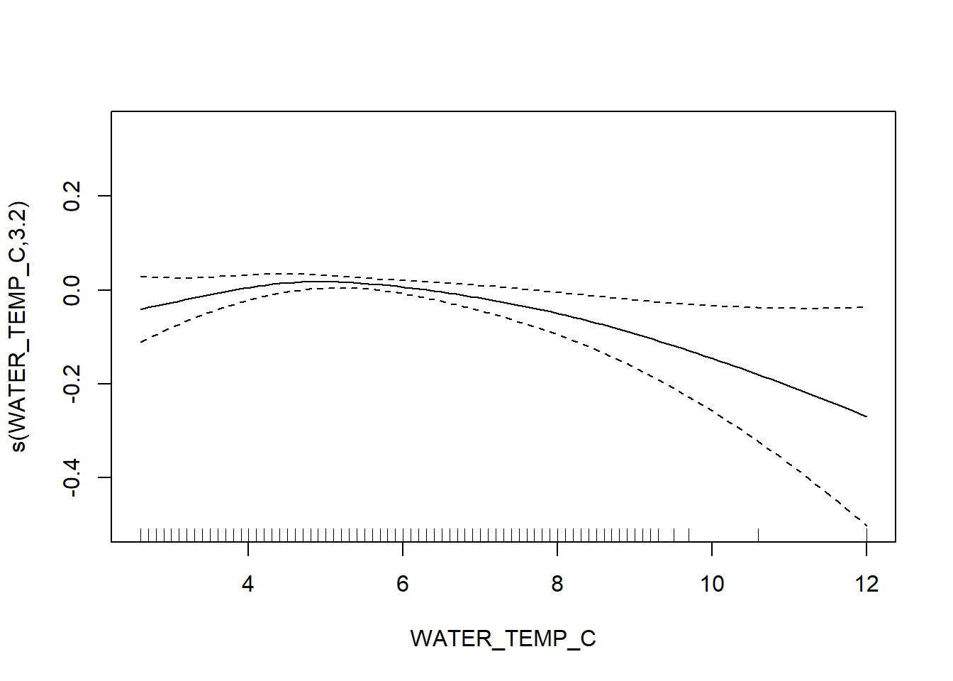


FVCOM data
delta_var_spring_FV <- gamm4(delta_var ~ s(FV_bot_temp) + s(FV_surf_temp) + s(FV_bot_sal) +  s(metric_tons) +   s(FV_surf_sal) +  s(START_DEPTH) + s(START_LATITUDE, START_LONGITUDE), random = ~ (1|YEAR) , data = spring_fvcom)

gam.check(delta_var_spring_FV$gam)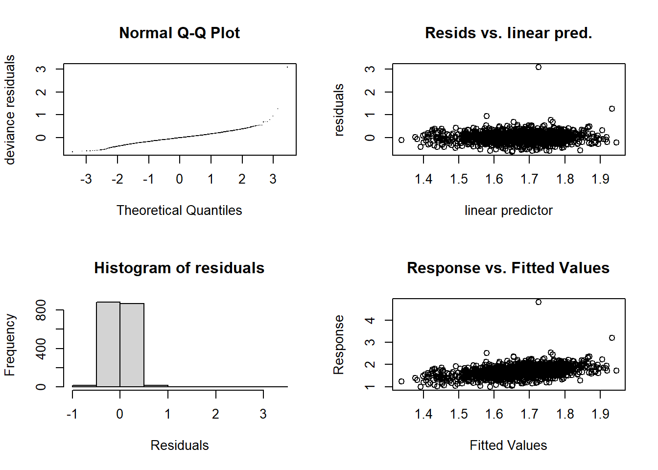
##
## 'gamm' based fit - care required with interpretation.
## Checks based on working residuals may be misleading.
## Basis dimension (k) checking results. Low p-value (k-index<1) may
## indicate that k is too low, especially if edf is close to k'.
##
##                                      k'   edf k-index p-value
## s(FV_bot_temp)                     9.00  3.76    1.04    0.94
## s(FV_surf_temp)                    9.00  1.21    0.99    0.28
## s(FV_bot_sal)                      9.00  1.00    0.97    0.10
## s(metric_tons)                     9.00  1.00    0.92  <2e-16 ***
## s(FV_surf_sal)                     9.00  1.00    1.02    0.87
## s(START_DEPTH)                     9.00  4.84    0.92  <2e-16 ***
## s(START_LATITUDE,START_LONGITUDE) 29.00 15.64    0.99    0.47
## ---
## Signif. codes: 0 '***' 0.001 '**' 0.01 '*' 0.05 '.' 0.1 ' ' 1summary(delta_var_spring_FV$gam)##
## Family: gaussian
## Link function: identity
##
## Formula:
## delta_var ~ s(FV_bot_temp) + s(FV_surf_temp) + s(FV_bot_sal) +
## s(metric_tons) + s(FV_surf_sal) + s(START_DEPTH) + s(START_LATITUDE,
## START_LONGITUDE)
##
## Parametric coefficients:
## Estimate Std. Error t value Pr(>|t|)
## (Intercept) 1.68340 0.01241 135.7 <2e-16 ***
## ---
## Signif. codes: 0 '***' 0.001 '**' 0.01 '*' 0.05 '.' 0.1 ' ' 1
##
## Approximate significance of smooth terms:
## edf Ref.df F p-value
## s(FV_bot_temp) 3.758 3.758 3.185 0.0143 *
## s(FV_surf_temp) 1.206 1.206 0.870 0.4250
## s(FV_bot_sal) 1.000 1.000 0.030 0.8634
## s(metric_tons) 1.000 1.000 1.084 0.2980
## s(FV_surf_sal) 1.000 1.000 3.610 0.0576 .
## s(START_DEPTH) 4.841 4.841 11.814 <2e-16 ***
## s(START_LATITUDE,START_LONGITUDE) 15.643 15.643 12.987 <2e-16 ***
## ---
## Signif. codes: 0 '***' 0.001 '**' 0.01 '*' 0.05 '.' 0.1 ' ' 1
##
## R-sq.(adj) = 0.179
## lmer.REML = -637.79 Scale est. = 0.037899 n = 1778plot(delta_var_spring_FV$gam)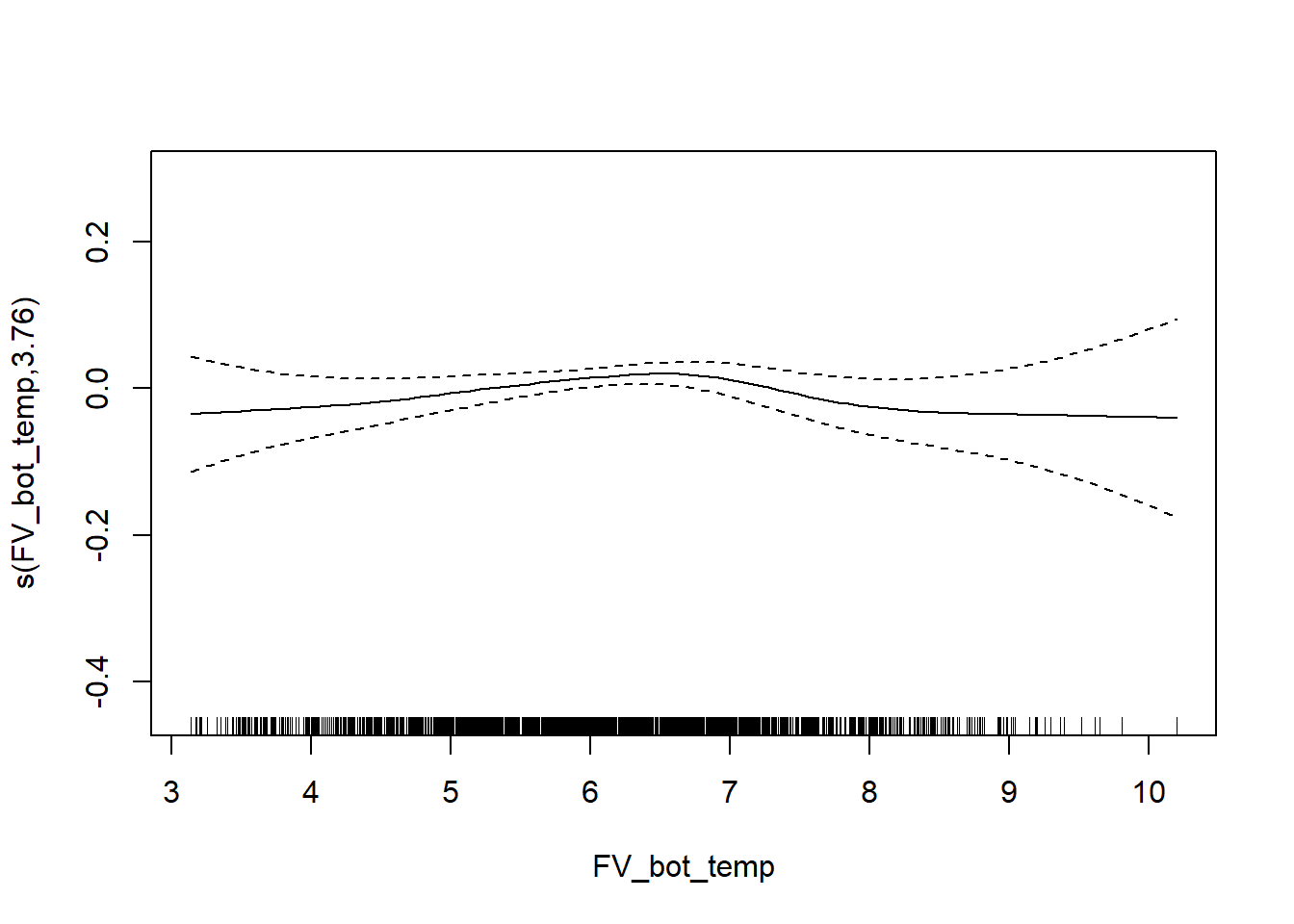
Fall GOM GAMMs
- all with FVCOM data
setwd("C:/Users/jjesse/Box/Kerr Lab/Fisheries Science Lab/ME NH Trawl- Seagrant/Seagrant-AEW/Results/GAMMs")

GOM_fall <- read.csv("GOM_fall_full.csv")

GOM_spring <- read.csv("GOM_spring_full.csv")
Species richness
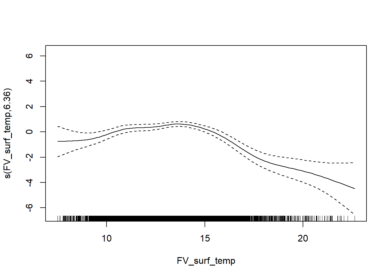
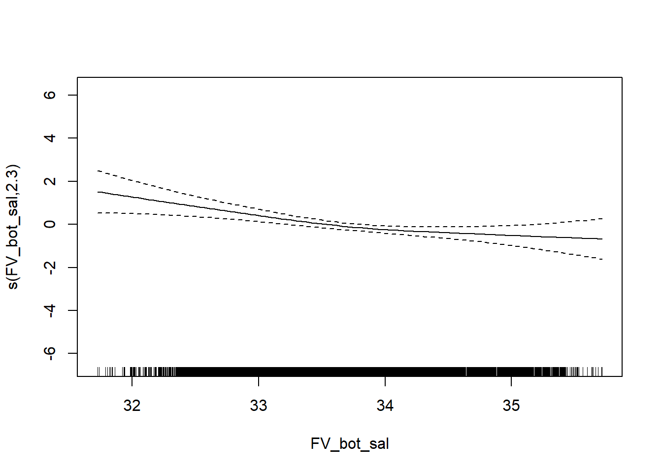
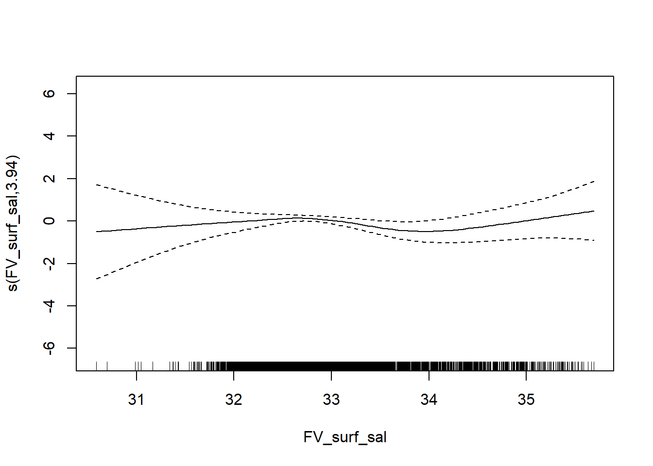
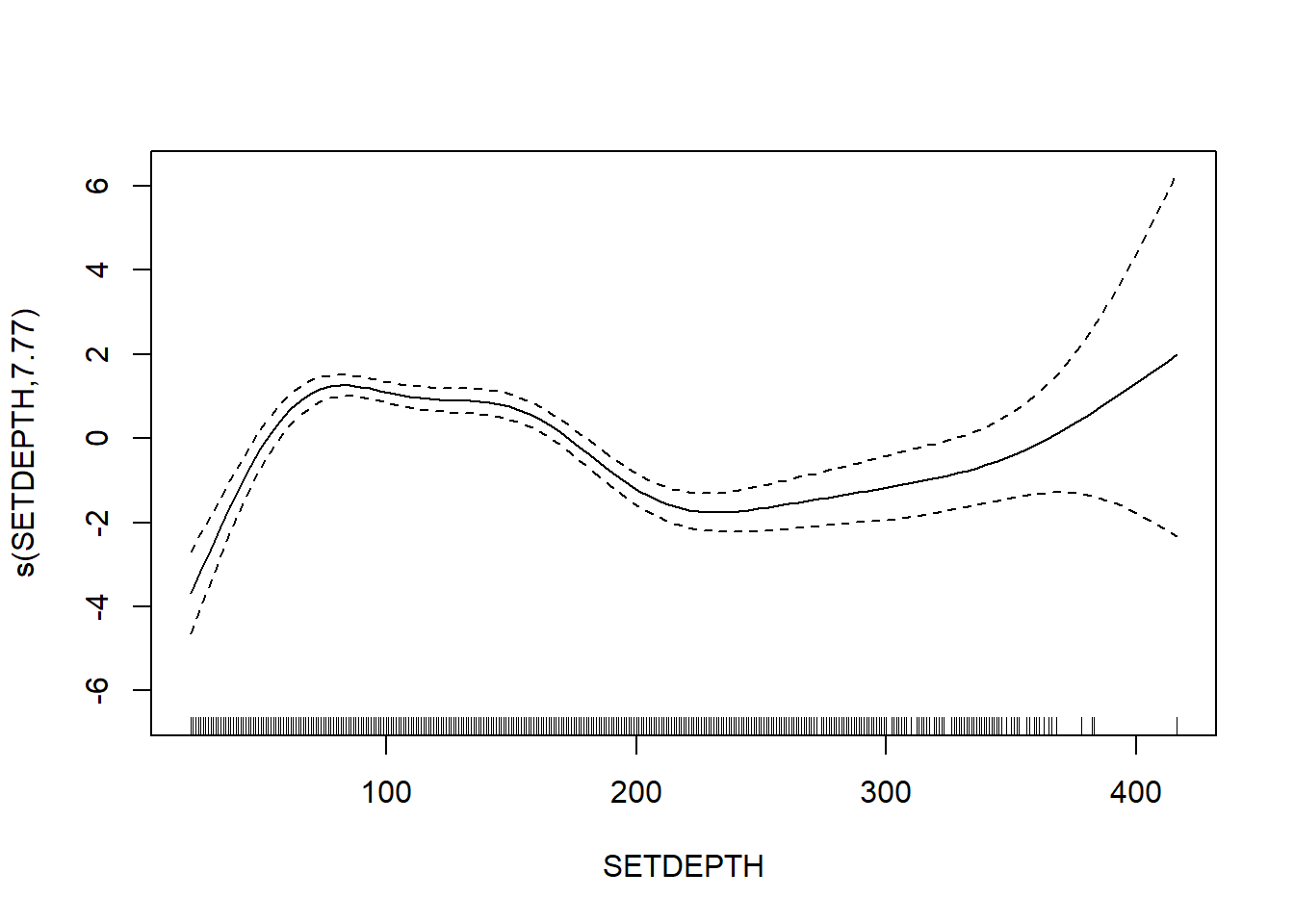
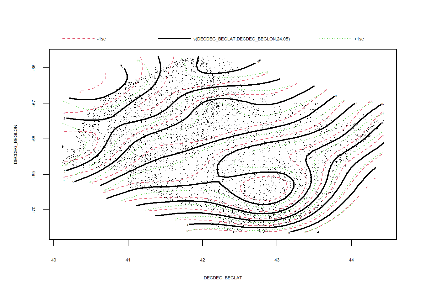
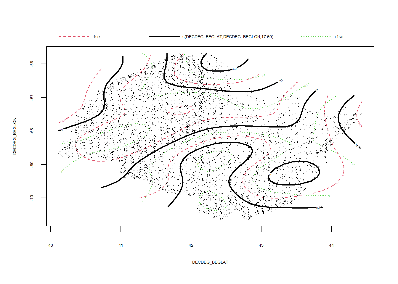
FV_GOM_N_FL <- gamm4(N_species ~ s(FV_bot_temp) + s(FV_surf_temp) + s(FV_bot_sal) +  s(FV_surf_sal) + s(SETDEPTH)+ s(DECDEG_BEGLAT, DECDEG_BEGLON) , random = ~ (1|EST_YEAR), data = GOM_fall)

gam.check(FV_GOM_N_FL$gam)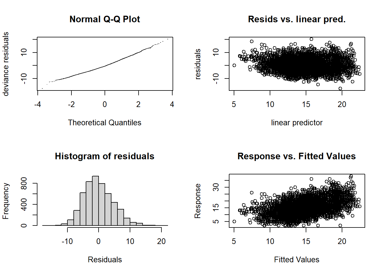
##
## 'gamm' based fit - care required with interpretation.
## Checks based on working residuals may be misleading.
## Basis dimension (k) checking results. Low p-value (k-index<1) may
## indicate that k is too low, especially if edf is close to k'.
##
##                                   k'   edf k-index p-value
## s(FV_bot_temp)                  9.00  5.41    0.95  <2e-16 ***
## s(FV_surf_temp)                 9.00  6.36    0.93  <2e-16 ***
## s(FV_bot_sal)                   9.00  2.30    1.01   0.705
## s(FV_surf_sal)                  9.00  3.94    0.96   0.005 **
## s(SETDEPTH)                     9.00  7.77    0.99   0.260
## s(DECDEG_BEGLAT,DECDEG_BEGLON) 29.00 24.05    0.98   0.040 *
## ---
## Signif. codes: 0 '***' 0.001 '**' 0.01 '*' 0.05 '.' 0.1 ' ' 1summary(FV_GOM_N_FL$gam)##
## Family: gaussian
## Link function: identity
##
## Formula:
## N_species ~ s(FV_bot_temp) + s(FV_surf_temp) + s(FV_bot_sal) +
## s(FV_surf_sal) + s(SETDEPTH) + s(DECDEG_BEGLAT, DECDEG_BEGLON)
##
## Parametric coefficients:
## Estimate Std. Error t value Pr(>|t|)
## (Intercept) 14.7045 0.5097 28.85 <2e-16 ***
## ---
## Signif. codes: 0 '***' 0.001 '**' 0.01 '*' 0.05 '.' 0.1 ' ' 1
##
## Approximate significance of smooth terms:
## edf Ref.df F p-value
## s(FV_bot_temp) 5.412 5.412 8.896 < 2e-16 ***
## s(FV_surf_temp) 6.362 6.362 18.933 < 2e-16 ***
## s(FV_bot_sal) 2.301 2.301 5.504 0.00251 **
## s(FV_surf_sal) 3.940 3.940 2.265 0.05737 .
## s(SETDEPTH) 7.771 7.771 32.328 < 2e-16 ***
## s(DECDEG_BEGLAT,DECDEG_BEGLON) 24.050 24.050 23.170 < 2e-16 ***
## ---
## Signif. codes: 0 '***' 0.001 '**' 0.01 '*' 0.05 '.' 0.1 ' ' 1
##
## R-sq.(adj) = 0.201
## lmer.REML = 27853 Scale est. = 11.485 n = 5215plot(FV_GOM_N_FL$gam)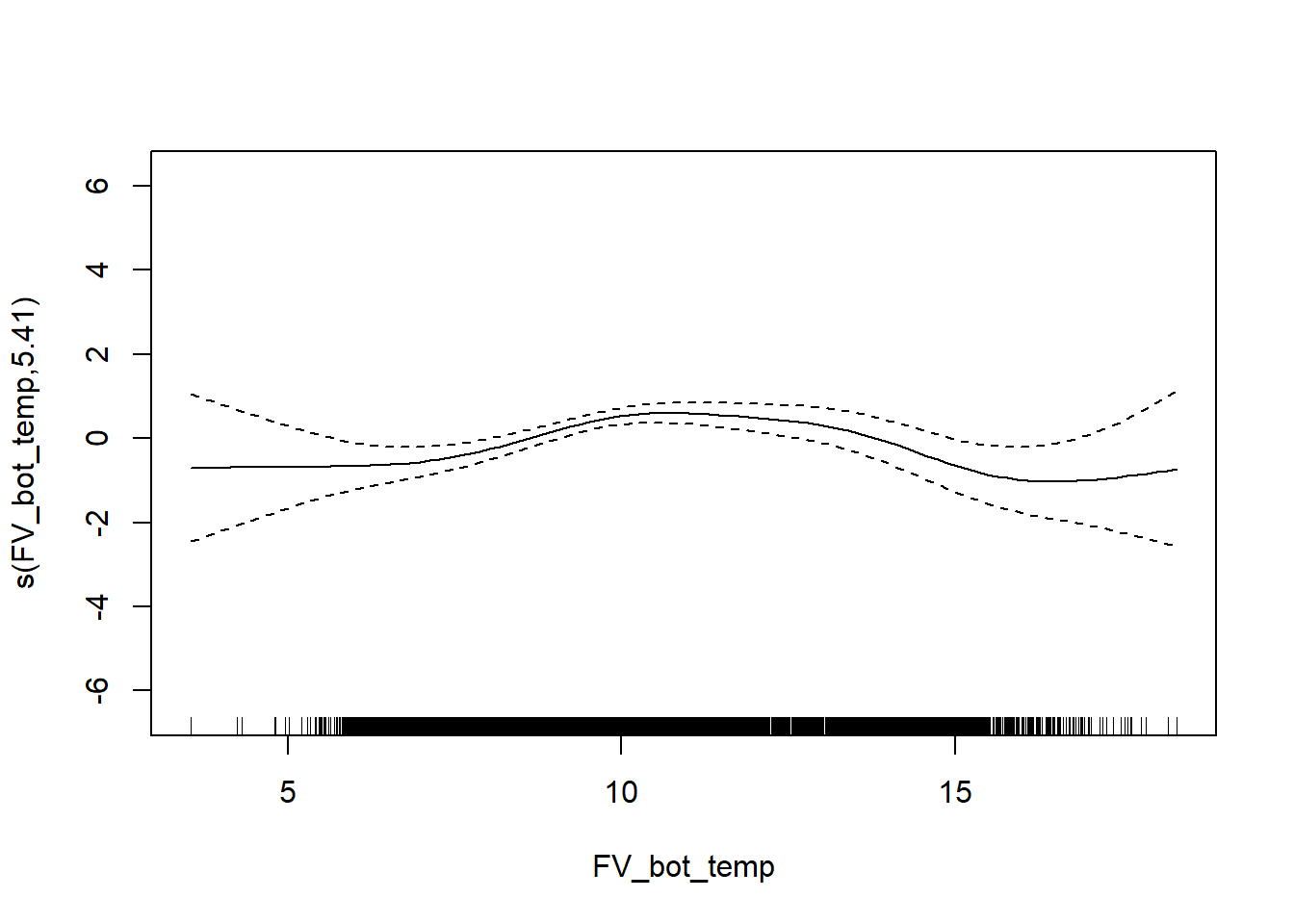
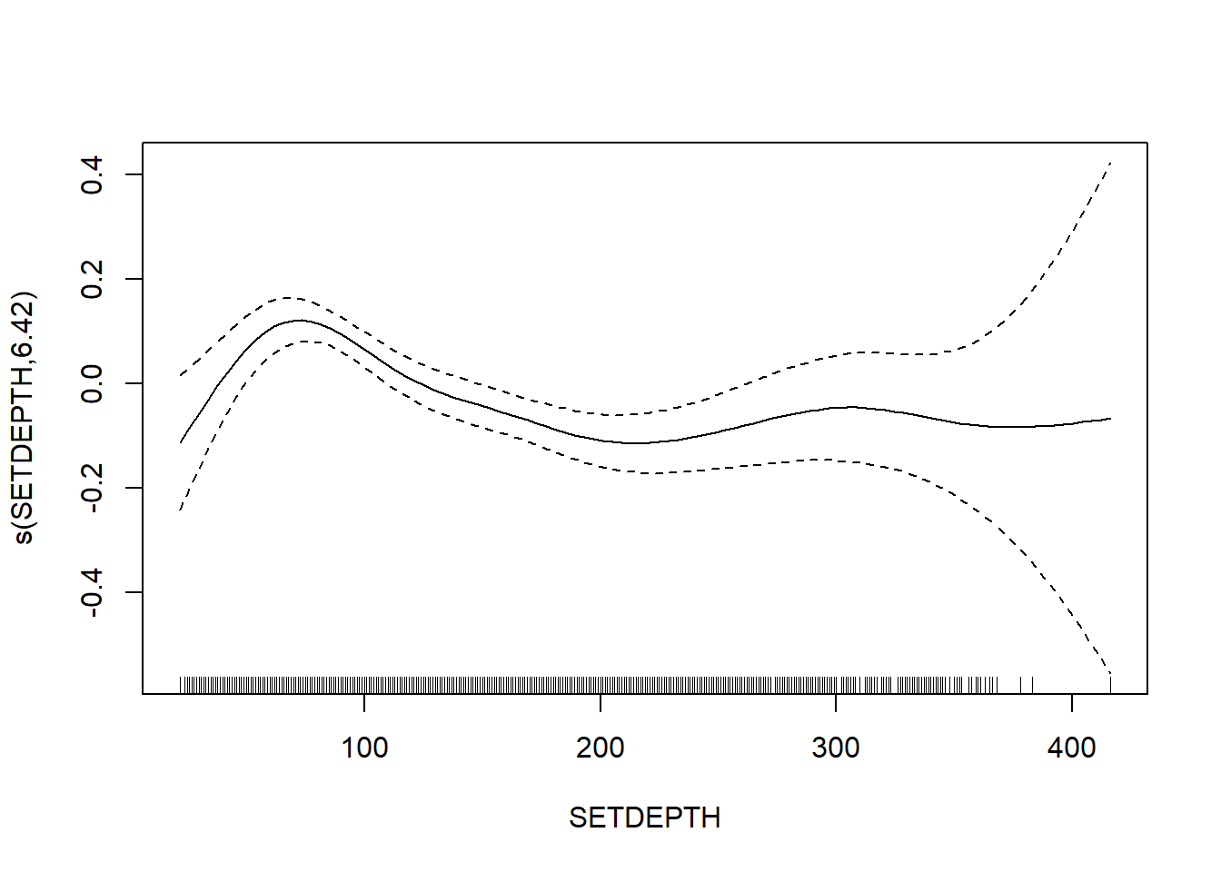
Shannon-Wiener
FV_GOM_H_FL <- gamm4(H_index ~ s(FV_bot_temp) + s(FV_surf_temp) + s(FV_bot_sal) +  s(FV_surf_sal) +  s(SETDEPTH)+ s(DECDEG_BEGLAT, DECDEG_BEGLON) , random = ~ (1|EST_YEAR), data = GOM_fall)

gam.check(FV_GOM_H_FL$gam)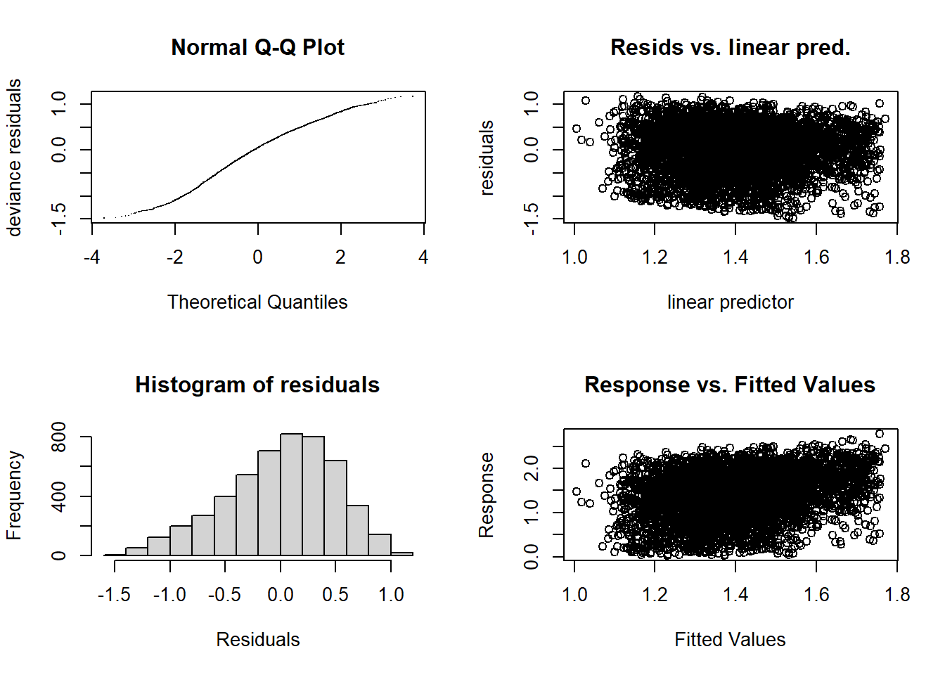
##
## 'gamm' based fit - care required with interpretation.
## Checks based on working residuals may be misleading.
## Basis dimension (k) checking results. Low p-value (k-index<1) may
## indicate that k is too low, especially if edf is close to k'.
##
##                                   k'   edf k-index p-value
## s(FV_bot_temp)                  9.00  5.38    0.98    0.07 .
## s(FV_surf_temp)                 9.00  3.84    1.00    0.44
## s(FV_bot_sal)                   9.00  5.61    1.00    0.59
## s(FV_surf_sal)                  9.00  3.87    1.01    0.66
## s(SETDEPTH)                     9.00  6.42    0.98    0.09 .
## s(DECDEG_BEGLAT,DECDEG_BEGLON) 29.00 17.69    0.99    0.23
## ---
## Signif. codes: 0 '***' 0.001 '**' 0.01 '*' 0.05 '.' 0.1 ' ' 1summary(FV_GOM_H_FL$gam)##
## Family: gaussian
## Link function: identity
##
## Formula:
## H_index ~ s(FV_bot_temp) + s(FV_surf_temp) + s(FV_bot_sal) +
## s(FV_surf_sal) + s(SETDEPTH) + s(DECDEG_BEGLAT, DECDEG_BEGLON)
##
## Parametric coefficients:
## Estimate Std. Error t value Pr(>|t|)
## (Intercept) 1.40982 0.01318 107 <2e-16 ***
## ---
## Signif. codes: 0 '***' 0.001 '**' 0.01 '*' 0.05 '.' 0.1 ' ' 1
##
## Approximate significance of smooth terms:
## edf Ref.df F p-value
## s(FV_bot_temp) 5.379 5.379 4.138 0.000411 ***
## s(FV_surf_temp) 3.845 3.845 1.071 0.243491
## s(FV_bot_sal) 5.610 5.610 3.877 0.000742 ***
## s(FV_surf_sal) 3.870 3.870 3.032 0.025389 *
## s(SETDEPTH) 6.420 6.420 7.528 < 2e-16 ***
## s(DECDEG_BEGLAT,DECDEG_BEGLON) 17.690 17.690 4.886 < 2e-16 ***
## ---
## Signif. codes: 0 '***' 0.001 '**' 0.01 '*' 0.05 '.' 0.1 ' ' 1
##
## R-sq.(adj) = 0.0768
## lmer.REML = 7272.6 Scale est. = 0.23797 n = 5055plot(FV_GOM_H_FL$gam)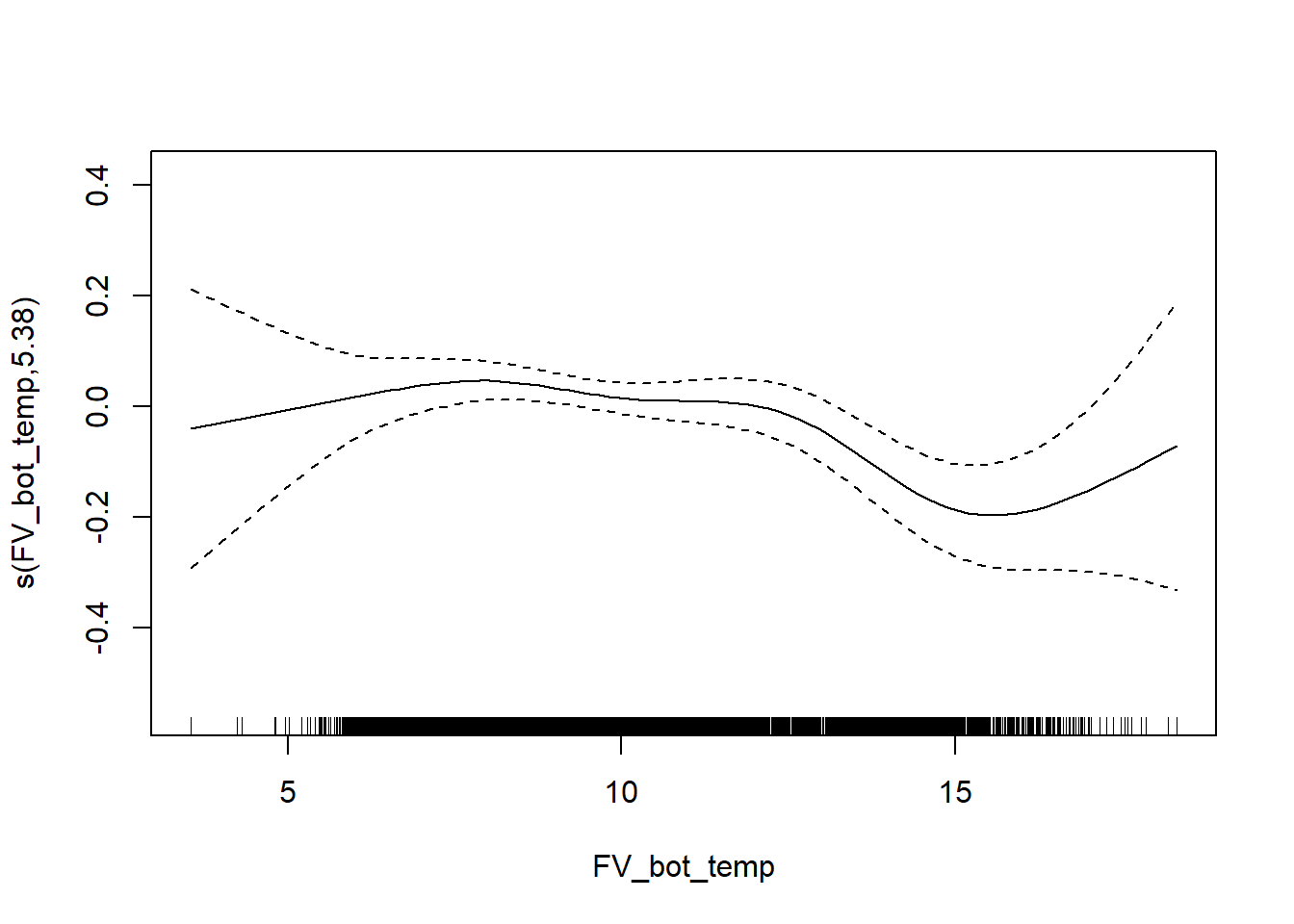
Simpson’s Dversity
FV_GOM_D_FL <- gamm4(D_index ~ s(FV_bot_temp) + s(FV_surf_temp) + s(FV_bot_sal) +  s(FV_surf_sal) + s(SETDEPTH)+ s(DECDEG_BEGLAT, DECDEG_BEGLON) , random = ~ (1|EST_YEAR), data = GOM_fall)

gam.check(FV_GOM_D_FL$gam)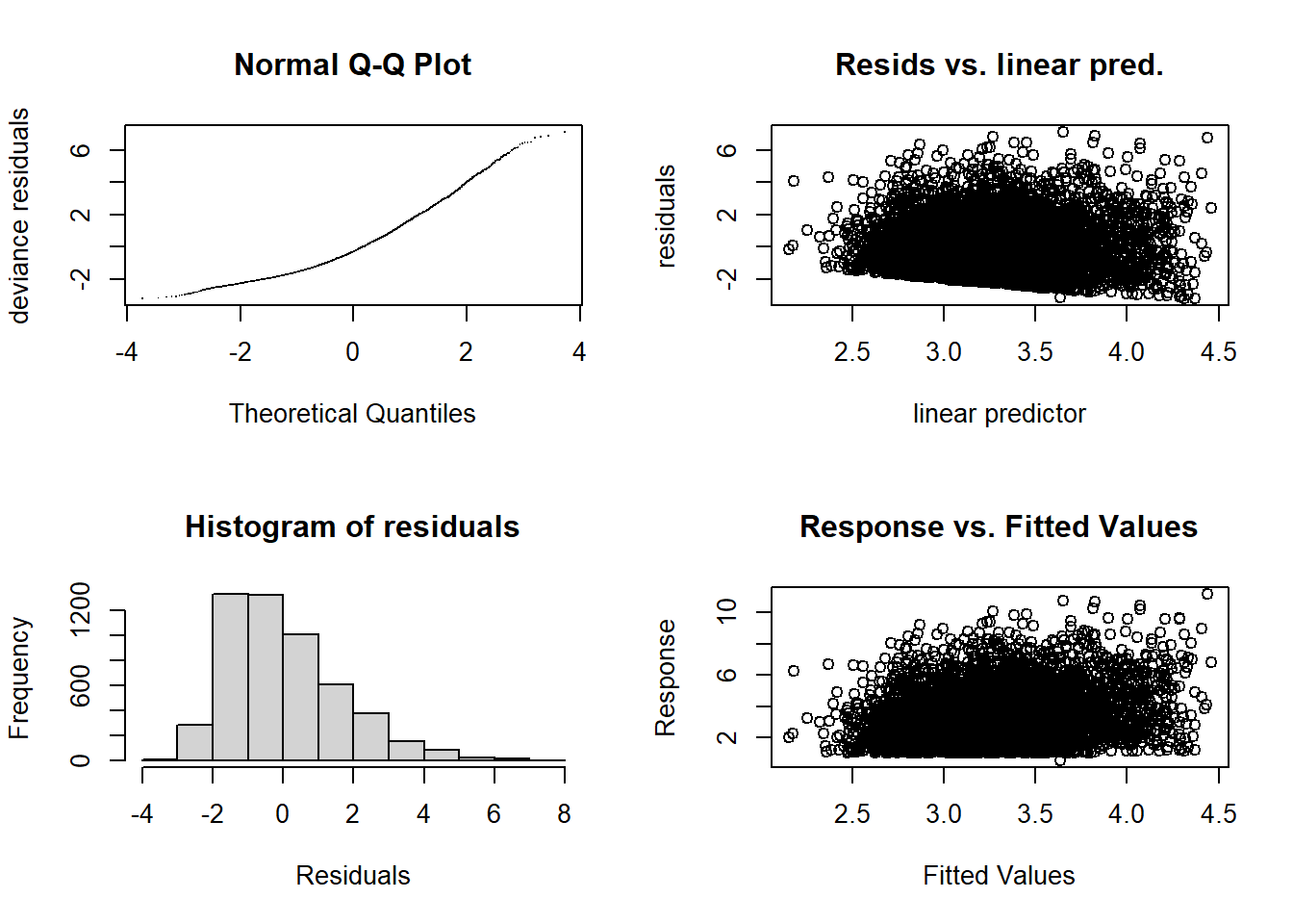
##
## 'gamm' based fit - care required with interpretation.
## Checks based on working residuals may be misleading.
## Basis dimension (k) checking results. Low p-value (k-index<1) may
## indicate that k is too low, especially if edf is close to k'.
##
##                                   k'   edf k-index p-value
## s(FV_bot_temp)                  9.00  2.43    0.99    0.30
## s(FV_surf_temp)                 9.00  3.52    0.99    0.32
## s(FV_bot_sal)                   9.00  4.85    0.99    0.20
## s(FV_surf_sal)                  9.00  3.21    1.01    0.70
## s(SETDEPTH)                     9.00  5.91    1.01    0.78
## s(DECDEG_BEGLAT,DECDEG_BEGLON) 29.00 14.48 0.99 0.19summary(FV_GOM_D_FL$gam)##
## Family: gaussian
## Link function: identity
##
## Formula:
## D_index ~ s(FV_bot_temp) + s(FV_surf_temp) + s(FV_bot_sal) +
## s(FV_surf_sal) + s(SETDEPTH) + s(DECDEG_BEGLAT, DECDEG_BEGLON)
##
## Parametric coefficients:
## Estimate Std. Error t value Pr(>|t|)
## (Intercept) 3.26844 0.04471 73.11 <2e-16 ***
## ---
## Signif. codes: 0 '***' 0.001 '**' 0.01 '*' 0.05 '.' 0.1 ' ' 1
##
## Approximate significance of smooth terms:
## edf Ref.df F p-value
## s(FV_bot_temp) 2.434 2.434 8.038 0.000154 ***
## s(FV_surf_temp) 3.523 3.523 0.675 0.415678
## s(FV_bot_sal) 4.853 4.853 4.186 0.001348 **
## s(FV_surf_sal) 3.213 3.213 1.852 0.176370
## s(SETDEPTH) 5.914 5.914 8.819 < 2e-16 ***
## s(DECDEG_BEGLAT,DECDEG_BEGLON) 14.484 14.484 3.743 1.83e-06 ***
## ---
## Signif. codes: 0 '***' 0.001 '**' 0.01 '*' 0.05 '.' 0.1 ' ' 1
##
## R-sq.(adj) = 0.058
## lmer.REML = 19847 Scale est. = 2.5627 n = 5214plot(FV_GOM_D_FL$gam)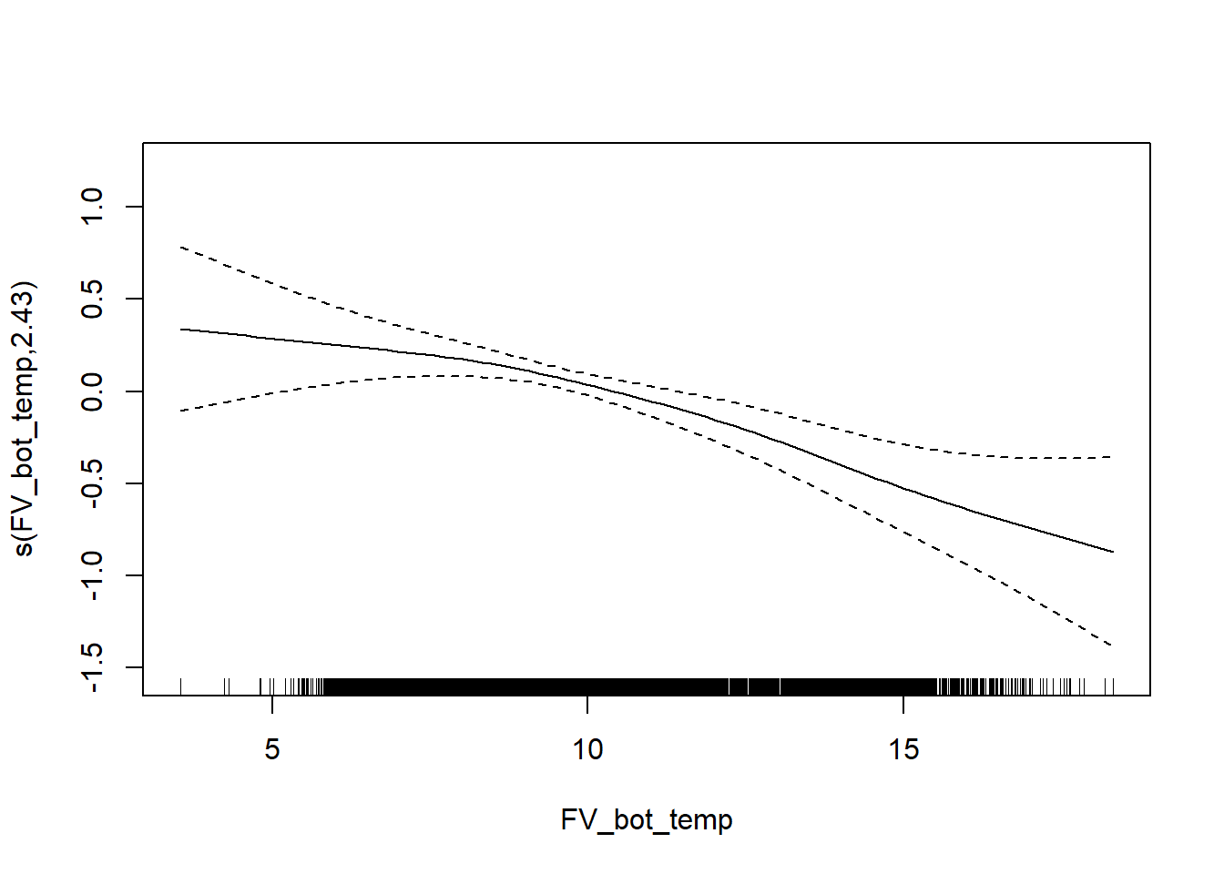
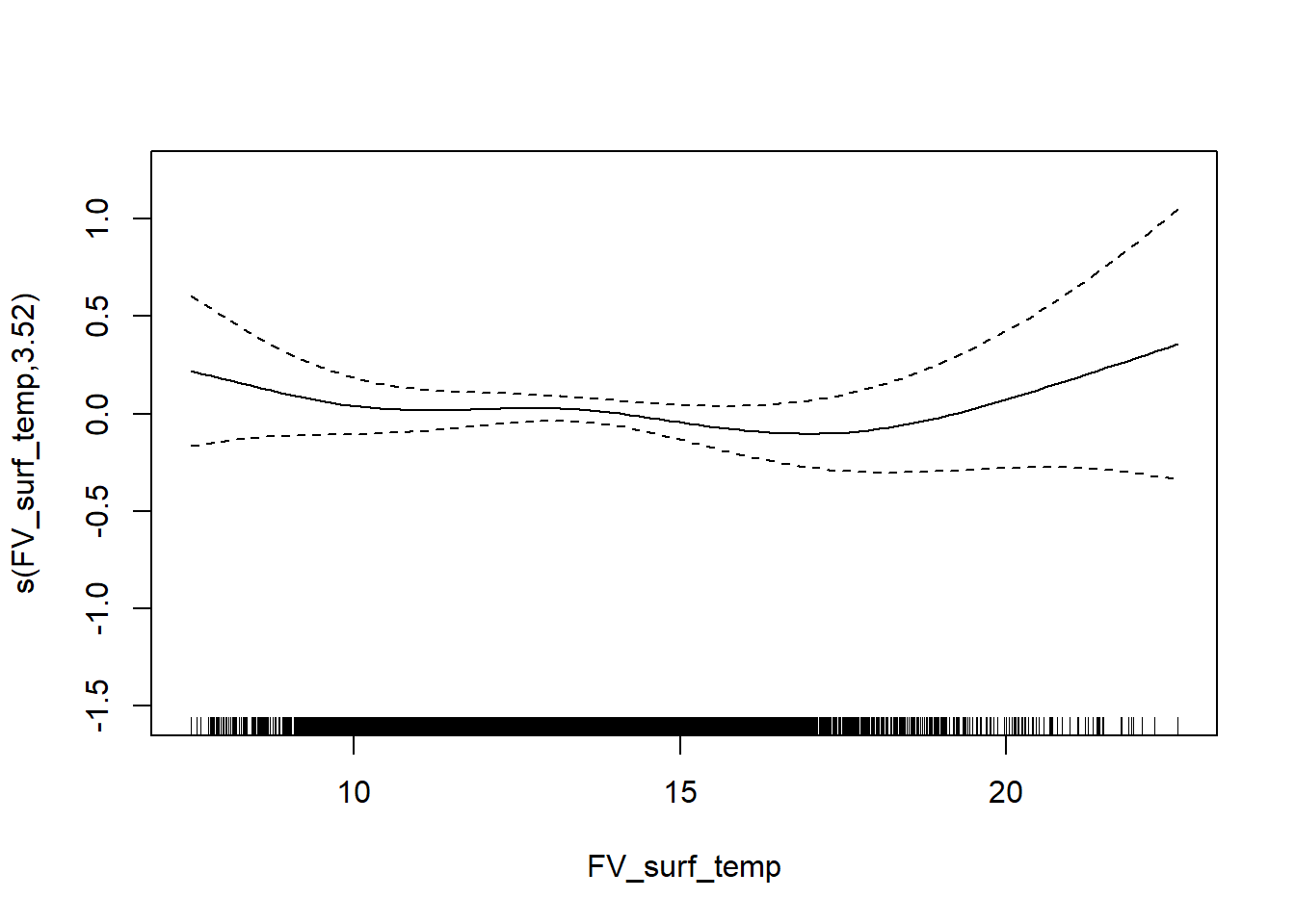
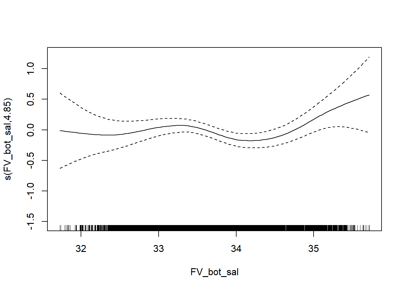
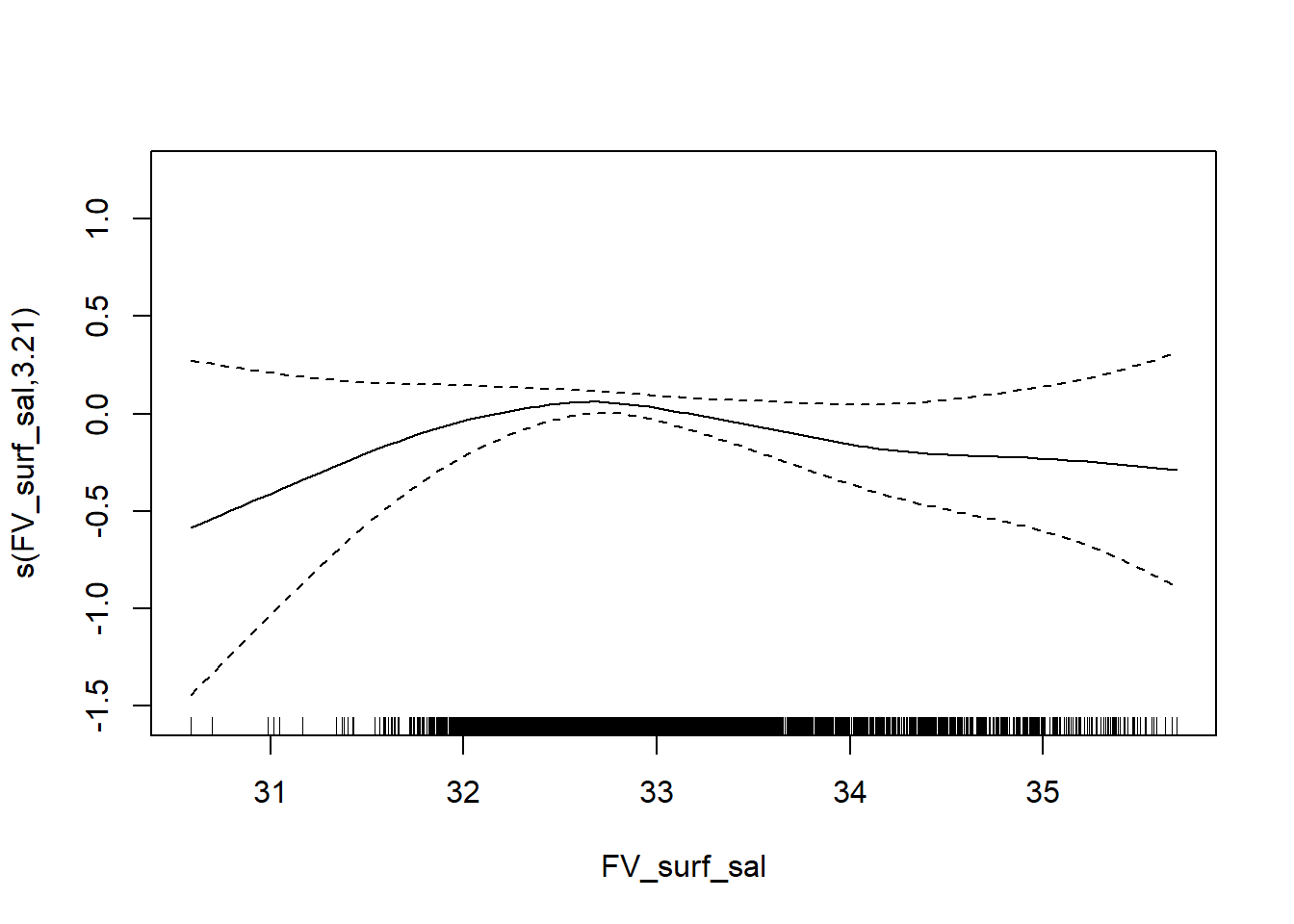
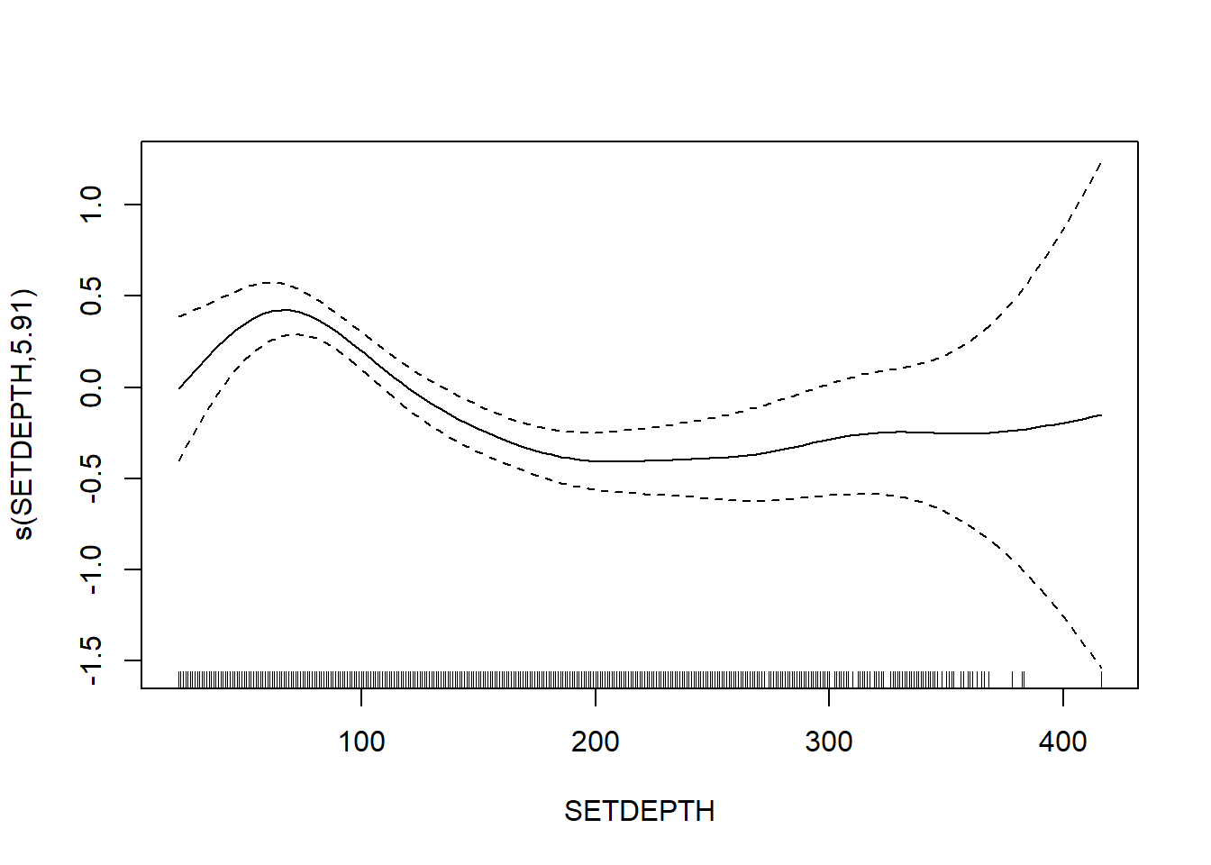
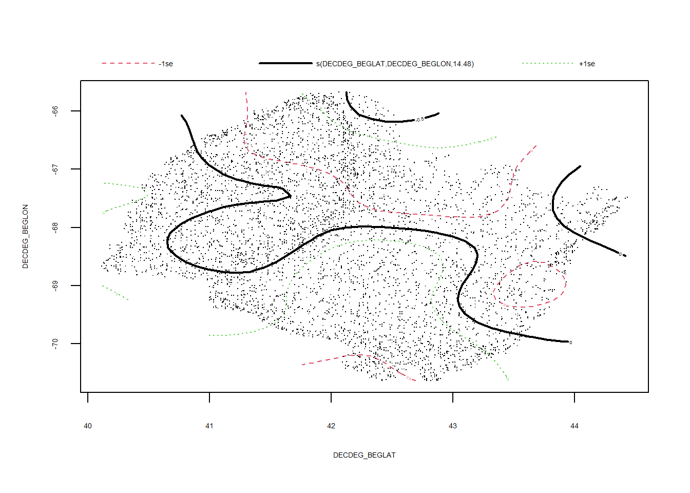
Simpson’s Evenness
FV_GOM_E_FL <- gamm4(E_index ~ s(FV_bot_temp) + s(FV_surf_temp) + s(FV_bot_sal) +  s(FV_surf_sal) +   s(SETDEPTH)+ s(DECDEG_BEGLAT, DECDEG_BEGLON) , random = ~ (1|EST_YEAR), data = GOM_fall)

gam.check(FV_GOM_E_FL$gam)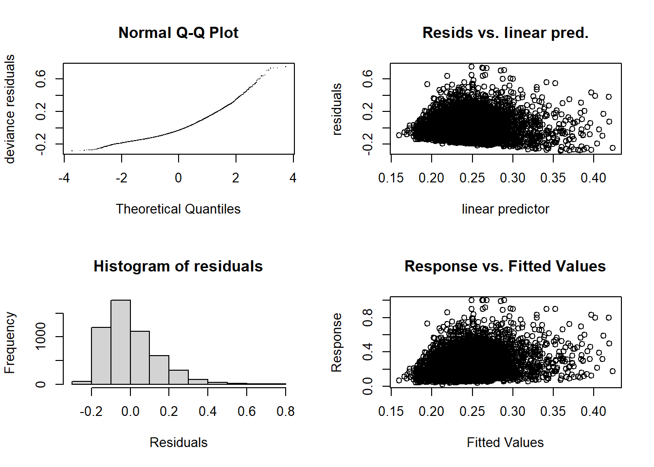
##
## 'gamm' based fit - care required with interpretation.
## Checks based on working residuals may be misleading.
## Basis dimension (k) checking results. Low p-value (k-index<1) may
## indicate that k is too low, especially if edf is close to k'.
##
##                                   k'   edf k-index p-value
## s(FV_bot_temp)                  9.00  1.00    0.99   0.160
## s(FV_surf_temp)                 9.00  3.58    0.98   0.035 *
## s(FV_bot_sal)                   9.00  5.06    0.99   0.230
## s(FV_surf_sal)                  9.00  1.08    0.99   0.340
## s(SETDEPTH)                     9.00  5.38    1.01   0.630
## s(DECDEG_BEGLAT,DECDEG_BEGLON) 29.00 14.33    0.99   0.160
## ---
## Signif. codes: 0 '***' 0.001 '**' 0.01 '*' 0.05 '.' 0.1 ' ' 1summary(FV_GOM_E_FL$gam)##
## Family: gaussian
## Link function: identity
##
## Formula:
## E_index ~ s(FV_bot_temp) + s(FV_surf_temp) + s(FV_bot_sal) +
## s(FV_surf_sal) + s(SETDEPTH) + s(DECDEG_BEGLAT, DECDEG_BEGLON)
##
## Parametric coefficients:
## Estimate Std. Error t value Pr(>|t|)
## (Intercept) 0.244586 0.009922 24.65 <2e-16 ***
## ---
## Signif. codes: 0 '***' 0.001 '**' 0.01 '*' 0.05 '.' 0.1 ' ' 1
##
## Approximate significance of smooth terms:
## edf Ref.df F p-value
## s(FV_bot_temp) 1.000 1.000 7.016 0.008101 **
## s(FV_surf_temp) 3.584 3.584 5.843 0.000291 ***
## s(FV_bot_sal) 5.060 5.060 3.381 0.005553 **
## s(FV_surf_sal) 1.079 1.079 0.068 0.810271
## s(SETDEPTH) 5.378 5.378 10.974 < 2e-16 ***
## s(DECDEG_BEGLAT,DECDEG_BEGLON) 14.330 14.330 4.264 < 2e-16 ***
## ---
## Signif. codes: 0 '***' 0.001 '**' 0.01 '*' 0.05 '.' 0.1 ' ' 1
##
## R-sq.(adj) = 0.0548
## lmer.REML = -6784.4 Scale est. = 0.015165 n = 5214plot(FV_GOM_E_FL$gam)
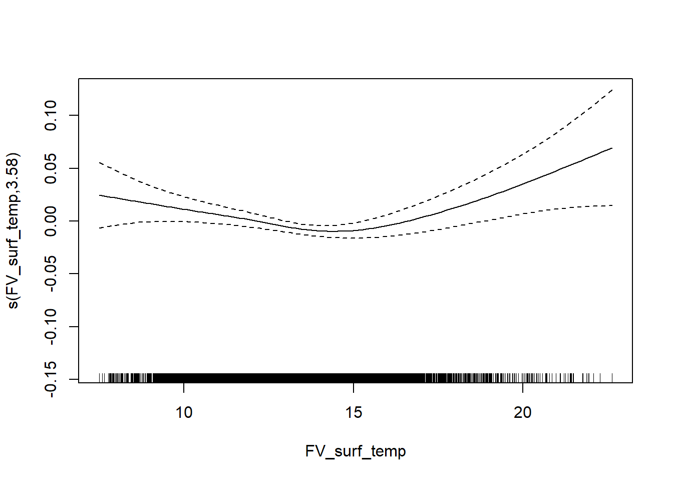
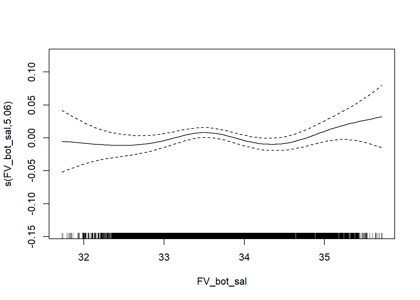
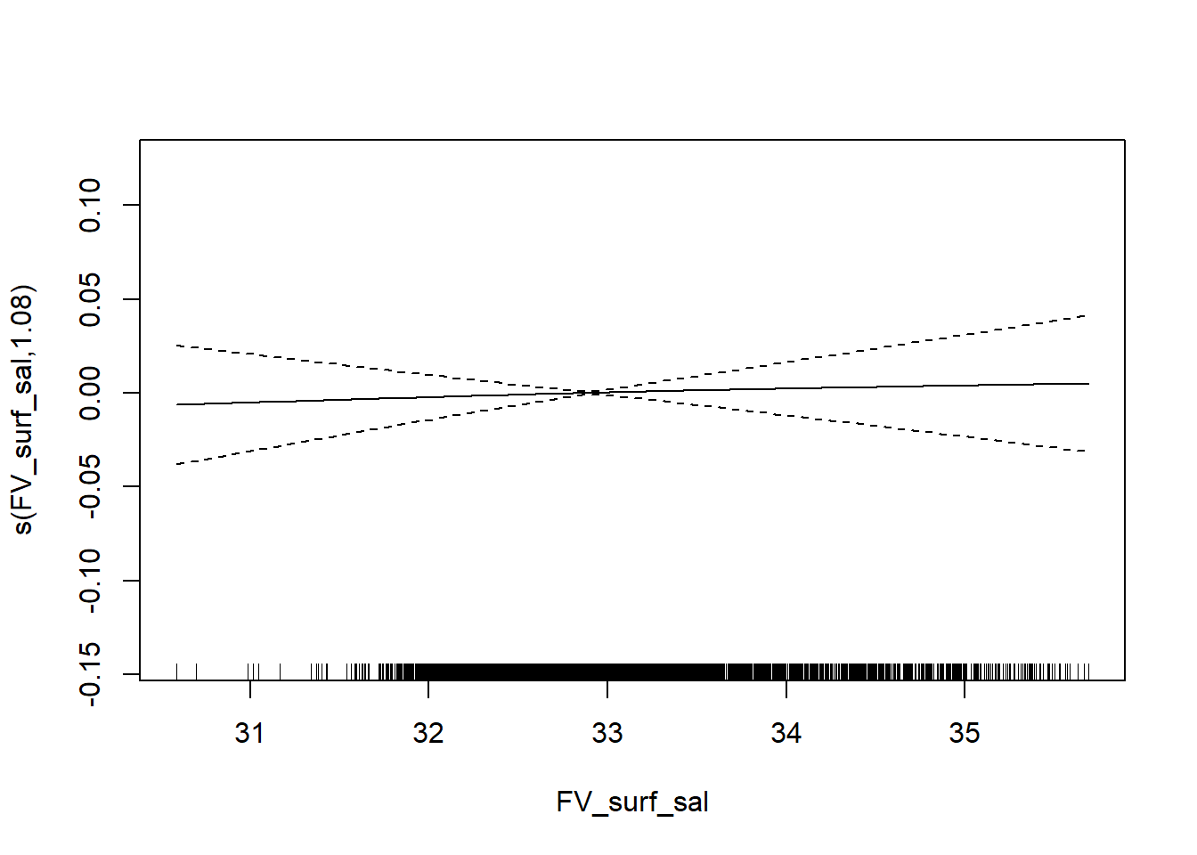
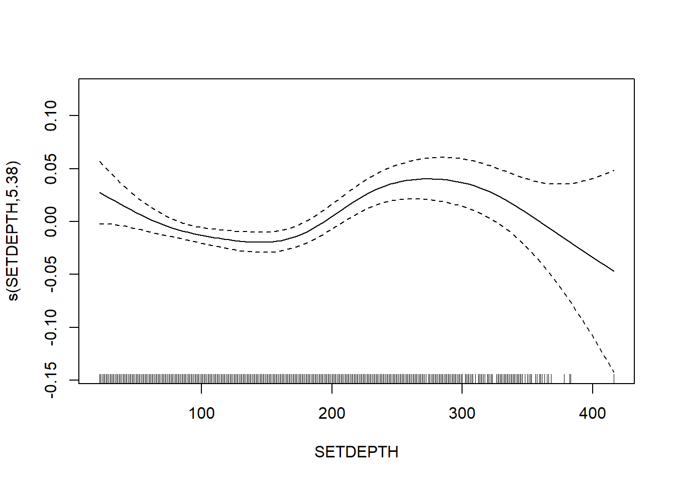
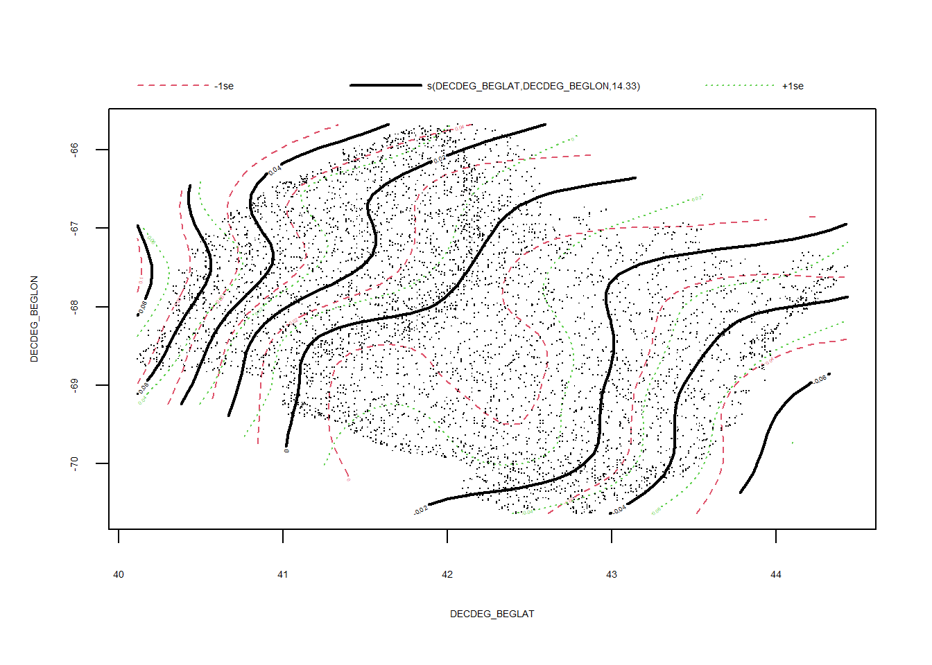
Taxonomic diversity
FV_GOM_delta_FL <- gamm4(delta ~ s(FV_bot_temp) + s(FV_surf_temp) + s(FV_bot_sal) +  s(FV_surf_sal) +  s(SETDEPTH)+ s(DECDEG_BEGLAT, DECDEG_BEGLON) , random = ~ (1|EST_YEAR), data = GOM_fall)

gam.check(FV_GOM_delta_FL$gam)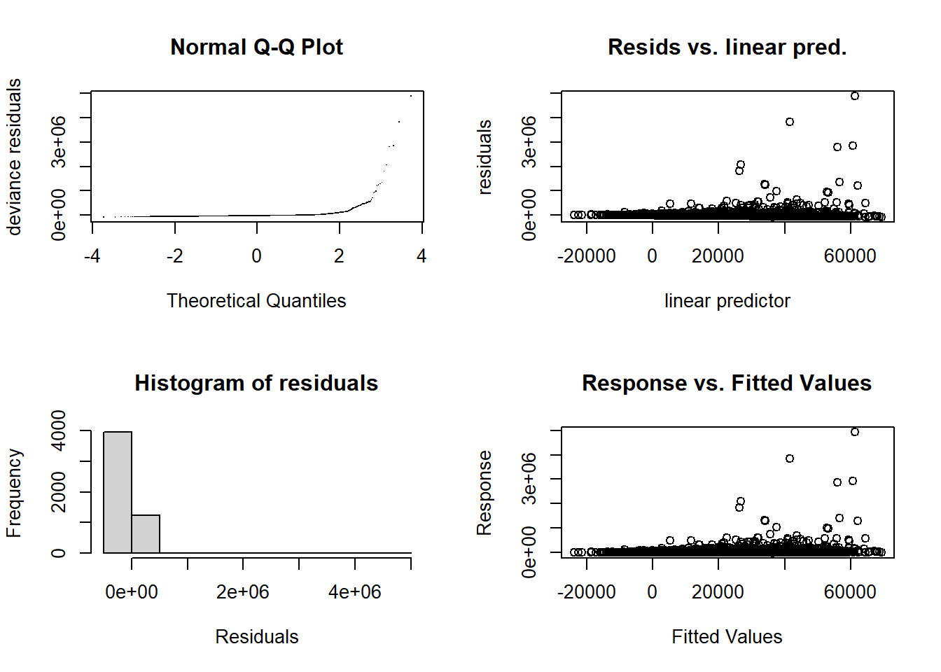
##
## 'gamm' based fit - care required with interpretation.
## Checks based on working residuals may be misleading.
## Basis dimension (k) checking results. Low p-value (k-index<1) may
## indicate that k is too low, especially if edf is close to k'.
##
##                                   k'   edf k-index p-value
## s(FV_bot_temp)                  9.00  1.29    1.00    0.62
## s(FV_surf_temp)                 9.00  1.00    1.00    0.26
## s(FV_bot_sal)                   9.00  2.81    1.00    0.34
## s(FV_surf_sal)                  9.00  1.52    1.00    0.29
## s(SETDEPTH)                     9.00  1.00    1.00    0.68
## s(DECDEG_BEGLAT,DECDEG_BEGLON) 29.00 9.42 1.07 0.79summary(FV_GOM_delta_FL$gam)##
## Family: gaussian
## Link function: identity
##
## Formula:
## delta ~ s(FV_bot_temp) + s(FV_surf_temp) + s(FV_bot_sal) + s(FV_surf_sal) +
## s(SETDEPTH) + s(DECDEG_BEGLAT, DECDEG_BEGLON)
##
## Parametric coefficients:
## Estimate Std. Error t value Pr(>|t|)
## (Intercept) 20444 4473 4.57 4.98e-06 ***
## ---
## Signif. codes: 0 '***' 0.001 '**' 0.01 '*' 0.05 '.' 0.1 ' ' 1
##
## Approximate significance of smooth terms:
## edf Ref.df F p-value
## s(FV_bot_temp) 1.288 1.288 1.975 0.2203
## s(FV_surf_temp) 1.000 1.000 4.901 0.0269 *
## s(FV_bot_sal) 2.807 2.807 2.408 0.0586 .
## s(FV_surf_sal) 1.524 1.524 2.196 0.1672
## s(SETDEPTH) 1.000 1.000 2.627 0.1051
## s(DECDEG_BEGLAT,DECDEG_BEGLON) 9.422 9.422 2.254 0.0116 *
## ---
## Signif. codes: 0 '***' 0.001 '**' 0.01 '*' 0.05 '.' 0.1 ' ' 1
##
## R-sq.(adj) = 0.0193
## lmer.REML = 1.3706e+05 Scale est. = 1.5374e+10 n = 5215plot(FV_GOM_delta_FL$gam)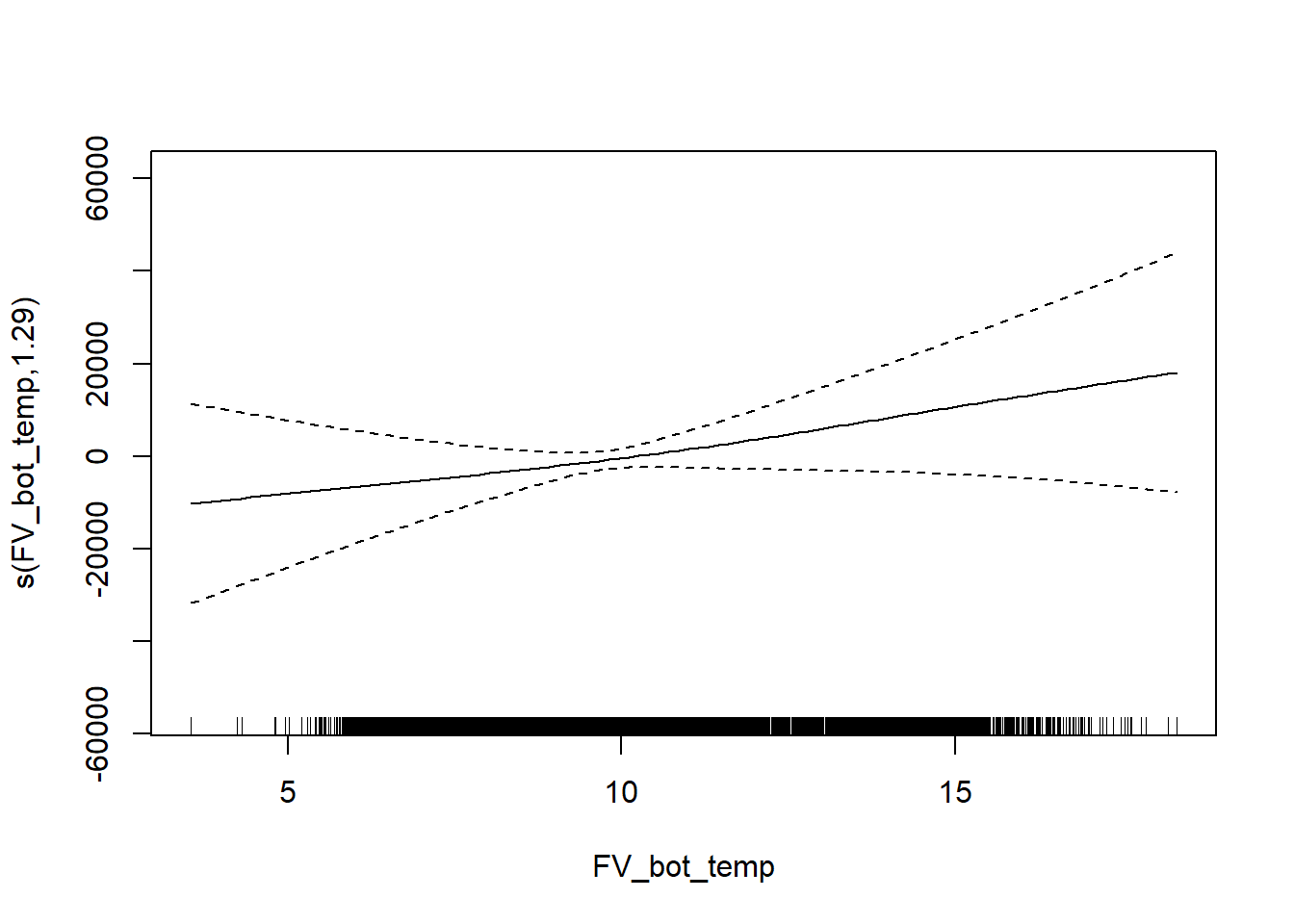
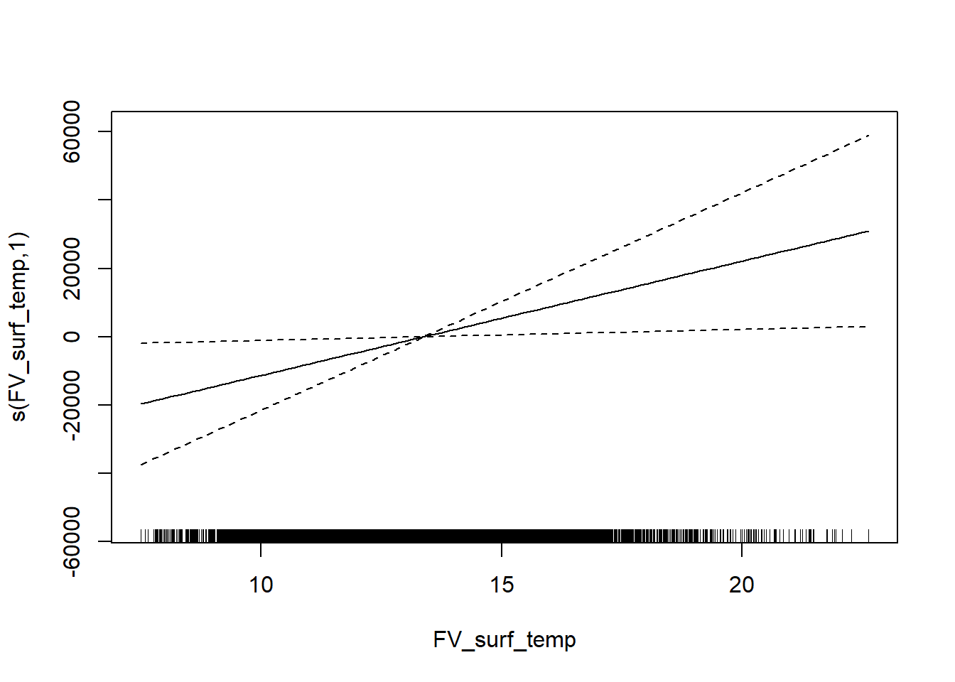
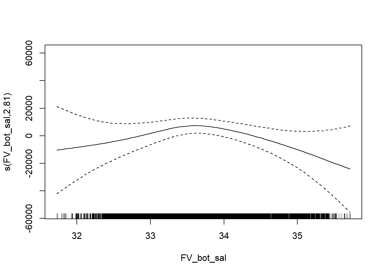
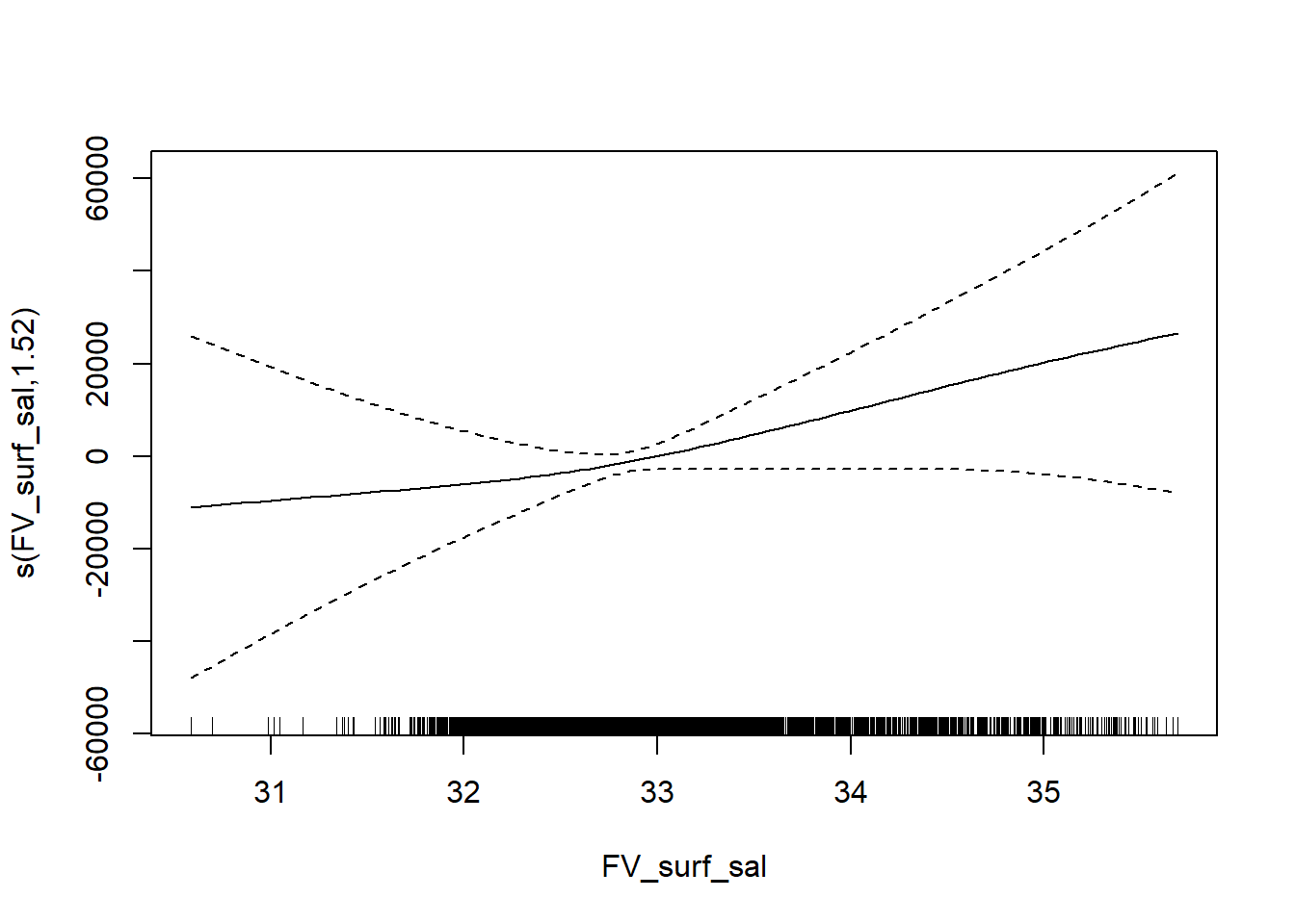
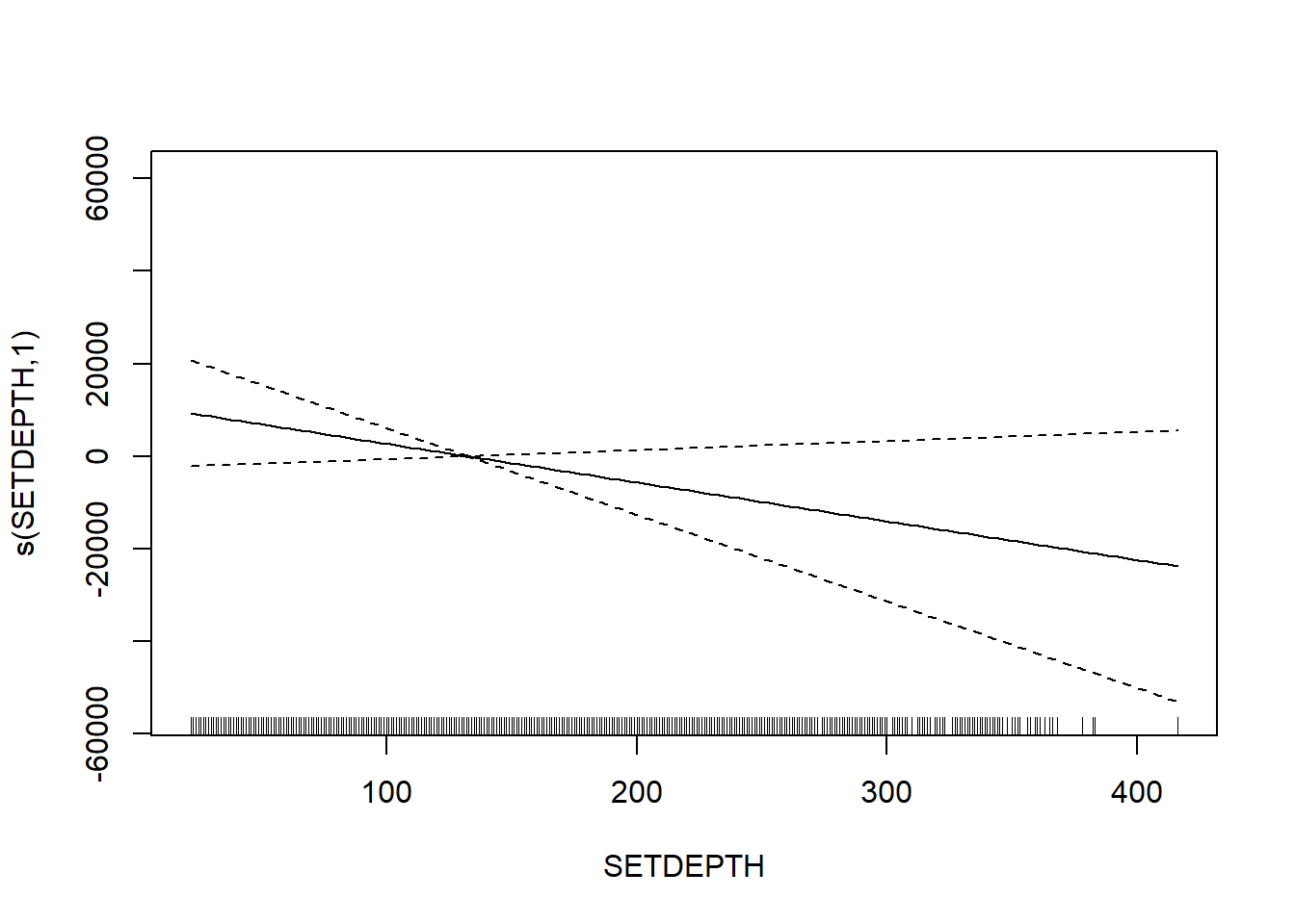
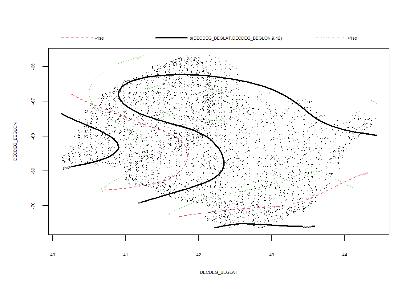
Taxonomic distinctness
FV_GOM_delta_star_FL <- gamm4(delta_star ~ s(FV_bot_temp) + s(FV_surf_temp) + s(FV_bot_sal) +  s(FV_surf_sal) +  s(SETDEPTH)+ s(DECDEG_BEGLAT, DECDEG_BEGLON) , random = ~ (1|EST_YEAR), data = GOM_fall)

gam.check(FV_GOM_delta_star_FL$gam)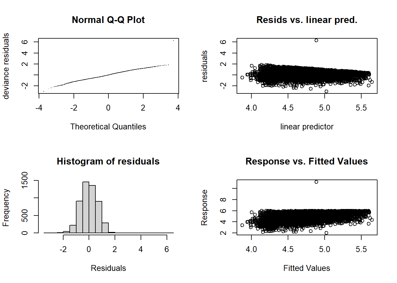
##
## 'gamm' based fit - care required with interpretation.
## Checks based on working residuals may be misleading.
## Basis dimension (k) checking results. Low p-value (k-index<1) may
## indicate that k is too low, especially if edf is close to k'.
##
##                                   k'   edf k-index p-value
## s(FV_bot_temp)                  9.00  5.65    1.00    0.46
## s(FV_surf_temp)                 9.00  2.47    1.01    0.76
## s(FV_bot_sal)                   9.00  1.67    0.97    0.03 *
## s(FV_surf_sal)                  9.00  3.34    0.99    0.22
## s(SETDEPTH)                     9.00  5.52    1.00    0.34
## s(DECDEG_BEGLAT,DECDEG_BEGLON) 29.00 23.15    0.93  <2e-16 ***
## ---
## Signif. codes: 0 '***' 0.001 '**' 0.01 '*' 0.05 '.' 0.1 ' ' 1summary(FV_GOM_delta_star_FL$gam)##
## Family: gaussian
## Link function: identity
##
## Formula:
## delta_star ~ s(FV_bot_temp) + s(FV_surf_temp) + s(FV_bot_sal) +
## s(FV_surf_sal) + s(SETDEPTH) + s(DECDEG_BEGLAT, DECDEG_BEGLON)
##
## Parametric coefficients:
## Estimate Std. Error t value Pr(>|t|)
## (Intercept) 4.71842 0.02346 201.1 <2e-16 ***
## ---
## Signif. codes: 0 '***' 0.001 '**' 0.01 '*' 0.05 '.' 0.1 ' ' 1
##
## Approximate significance of smooth terms:
## edf Ref.df F p-value
## s(FV_bot_temp) 5.655 5.655 17.267 < 2e-16 ***
## s(FV_surf_temp) 2.473 2.473 1.066 0.25599
## s(FV_bot_sal) 1.674 1.674 2.878 0.04209 *
## s(FV_surf_sal) 3.336 3.336 4.461 0.00249 **
## s(SETDEPTH) 5.524 5.524 13.605 < 2e-16 ***
## s(DECDEG_BEGLAT,DECDEG_BEGLON) 23.148 23.148 20.037 < 2e-16 ***
## ---
## Signif. codes: 0 '***' 0.001 '**' 0.01 '*' 0.05 '.' 0.1 ' ' 1
##
## R-sq.(adj) = 0.198
## lmer.REML = 10283 Scale est. = 0.40419 n = 5214plot(FV_GOM_delta_star_FL$gam)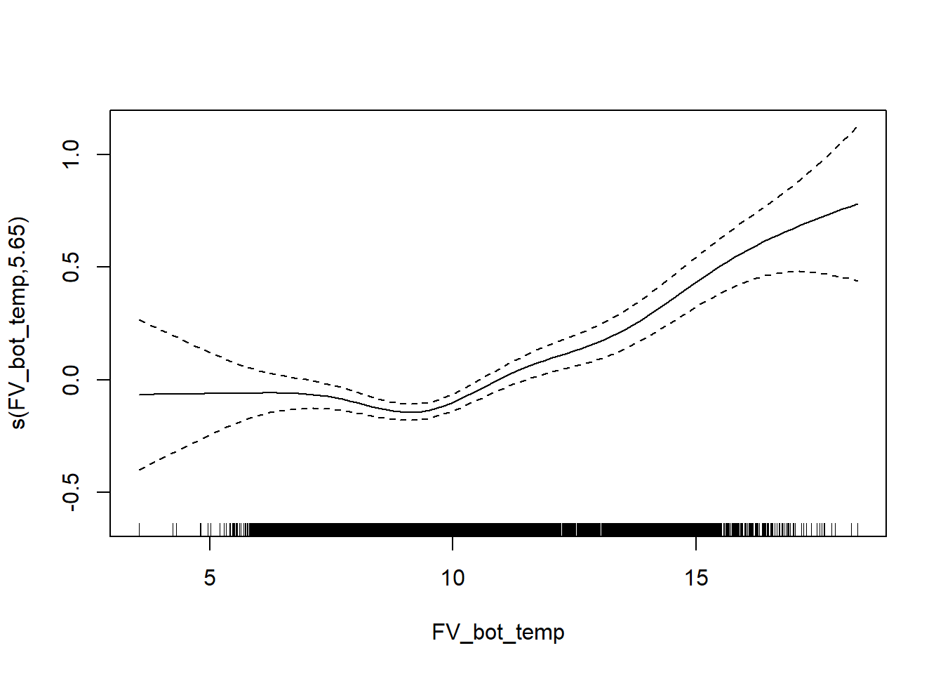
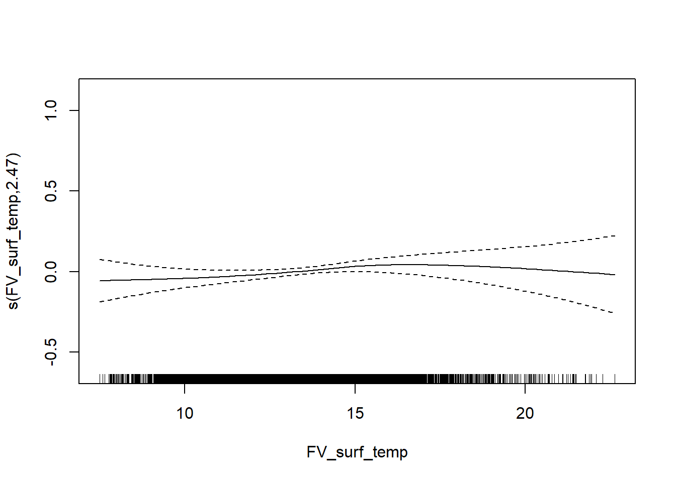
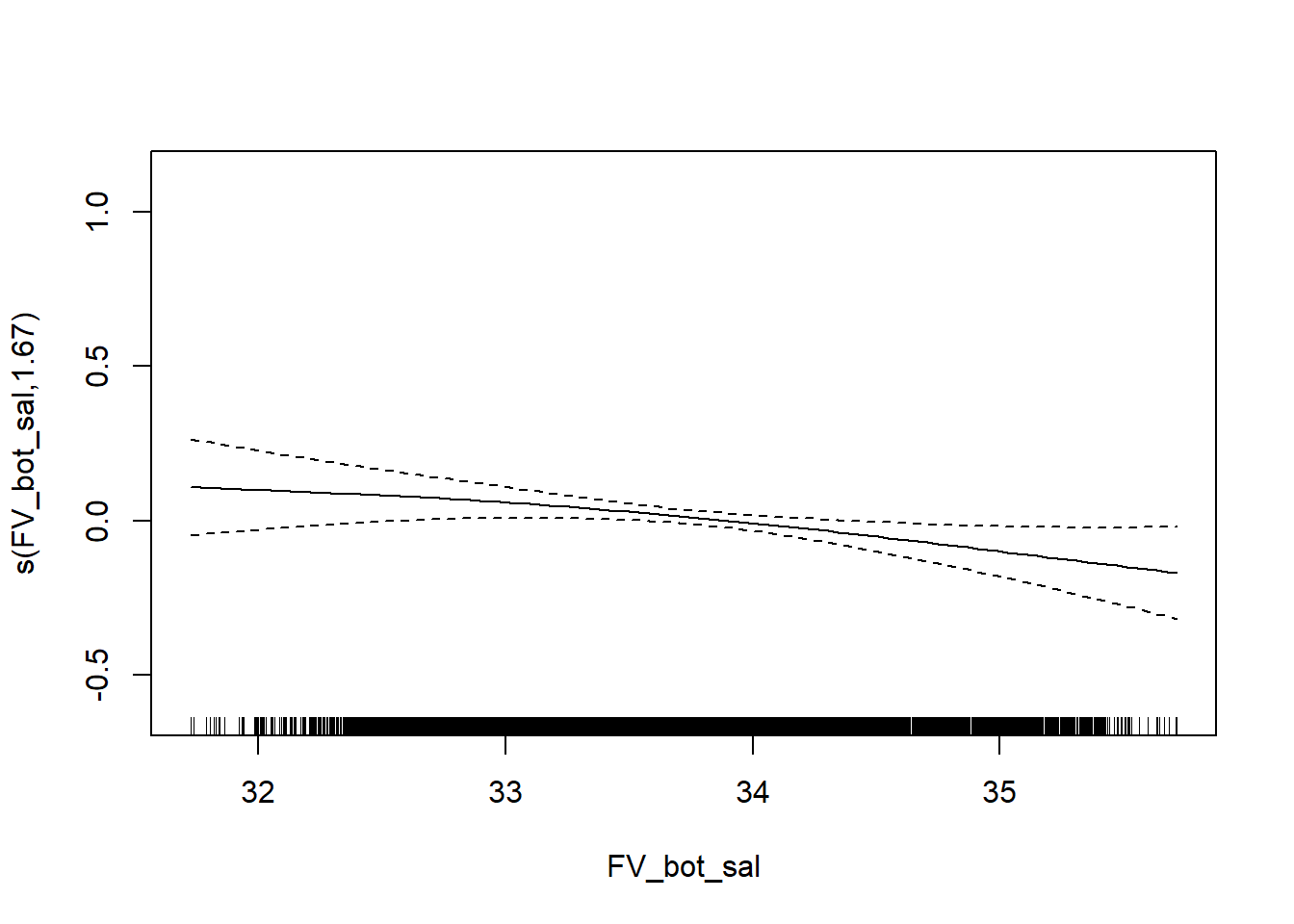
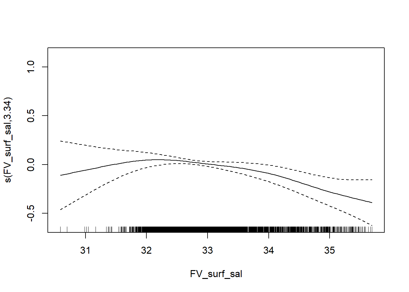
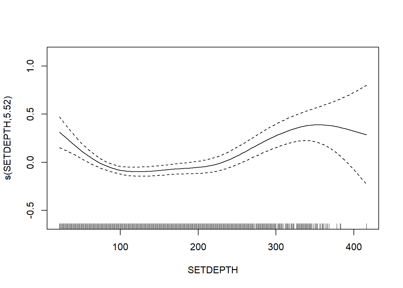
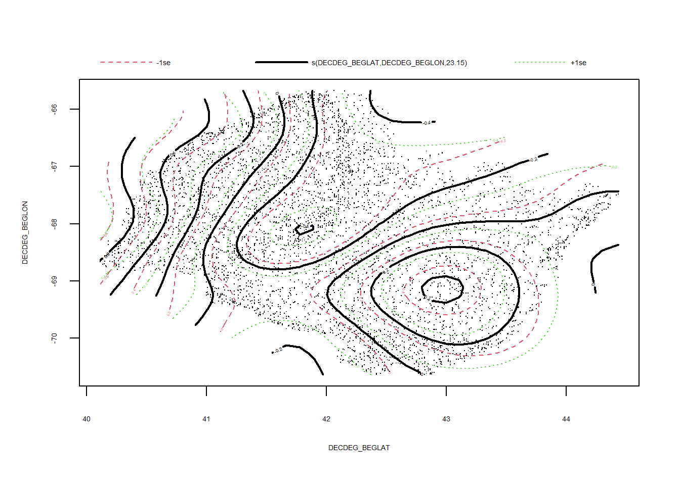
Average taxonomic distinctness
FV_GOM_delta_plus_FL <- gamm4(delta_plus ~ s(FV_bot_temp) + s(FV_surf_temp) + s(FV_bot_sal) +  s(FV_surf_sal) +  s(SETDEPTH)+ s(DECDEG_BEGLAT, DECDEG_BEGLON) , random = ~ (1|EST_YEAR), data = GOM_fall)

gam.check(FV_GOM_delta_plus_FL$gam)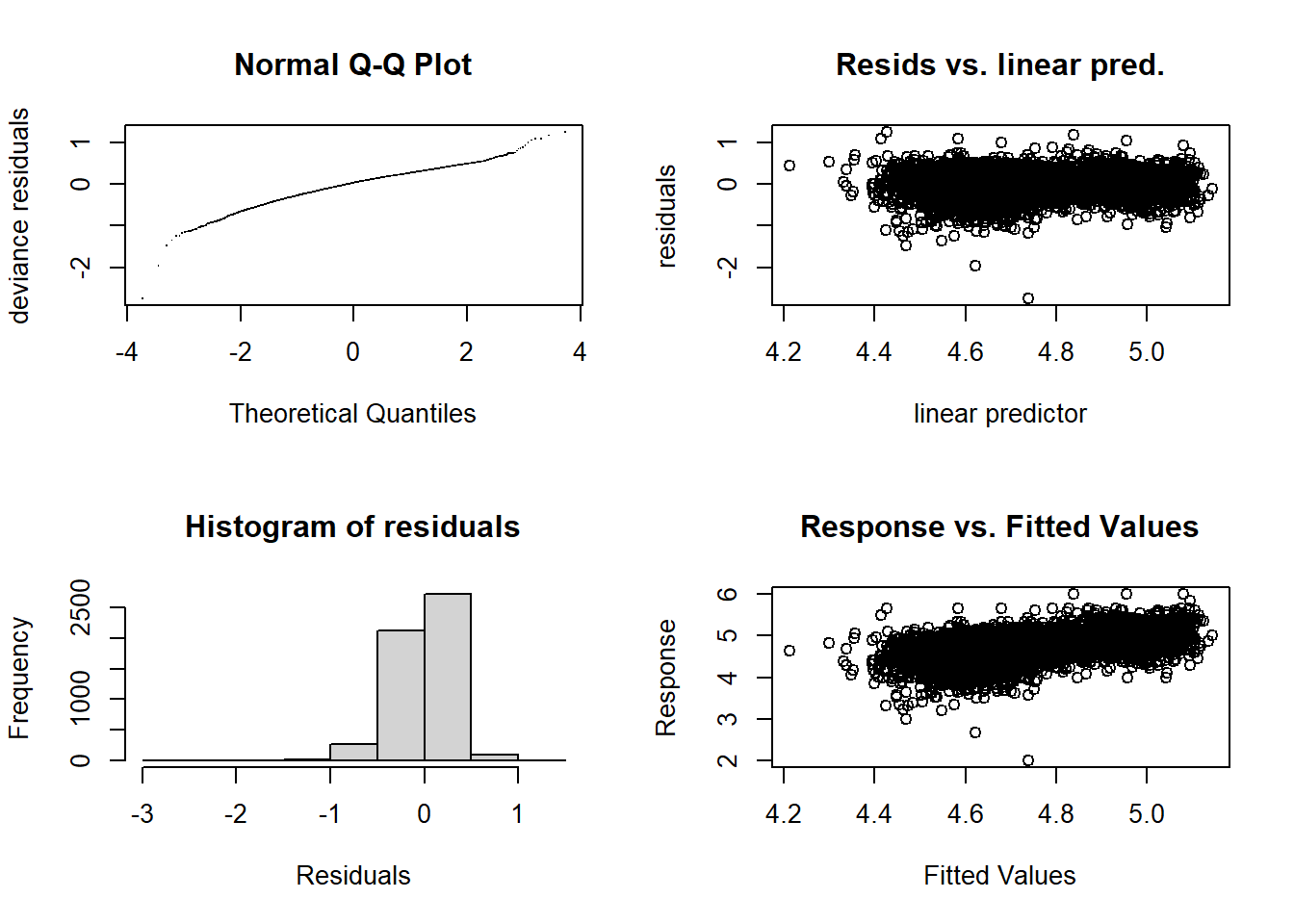
##
## 'gamm' based fit - care required with interpretation.
## Checks based on working residuals may be misleading.
## Basis dimension (k) checking results. Low p-value (k-index<1) may
## indicate that k is too low, especially if edf is close to k'.
##
##                                   k'   edf k-index p-value
## s(FV_bot_temp)                  9.00  4.69    0.96    0.01 **
## s(FV_surf_temp)                 9.00  3.70    0.97    0.04 *
## s(FV_bot_sal)                   9.00  3.56    1.00    0.56
## s(FV_surf_sal)                  9.00  1.00    1.00    0.64
## s(SETDEPTH)                     9.00  5.64    0.99    0.30
## s(DECDEG_BEGLAT,DECDEG_BEGLON) 29.00 23.02    0.98    0.09 .
## ---
## Signif. codes: 0 '***' 0.001 '**' 0.01 '*' 0.05 '.' 0.1 ' ' 1summary(FV_GOM_delta_plus_FL$gam)##
## Family: gaussian
## Link function: identity
##
## Formula:
## delta_plus ~ s(FV_bot_temp) + s(FV_surf_temp) + s(FV_bot_sal) +
## s(FV_surf_sal) + s(SETDEPTH) + s(DECDEG_BEGLAT, DECDEG_BEGLON)
##
## Parametric coefficients:
## Estimate Std. Error t value Pr(>|t|)
## (Intercept) 4.74830 0.01622 292.7 <2e-16 ***
## ---
## Signif. codes: 0 '***' 0.001 '**' 0.01 '*' 0.05 '.' 0.1 ' ' 1
##
## Approximate significance of smooth terms:
## edf Ref.df F p-value
## s(FV_bot_temp) 4.692 4.692 14.223 < 2e-16 ***
## s(FV_surf_temp) 3.703 3.703 6.543 7.44e-05 ***
## s(FV_bot_sal) 3.559 3.559 1.605 0.122
## s(FV_surf_sal) 1.000 1.000 0.210 0.647
## s(SETDEPTH) 5.643 5.643 19.312 < 2e-16 ***
## s(DECDEG_BEGLAT,DECDEG_BEGLON) 23.024 23.024 20.796 < 2e-16 ***
## ---
## Signif. codes: 0 '***' 0.001 '**' 0.01 '*' 0.05 '.' 0.1 ' ' 1
##
## R-sq.(adj) = 0.255
## lmer.REML = 1585.4 Scale est. = 0.07552 n = 5215plot(FV_GOM_delta_plus_FL$gam)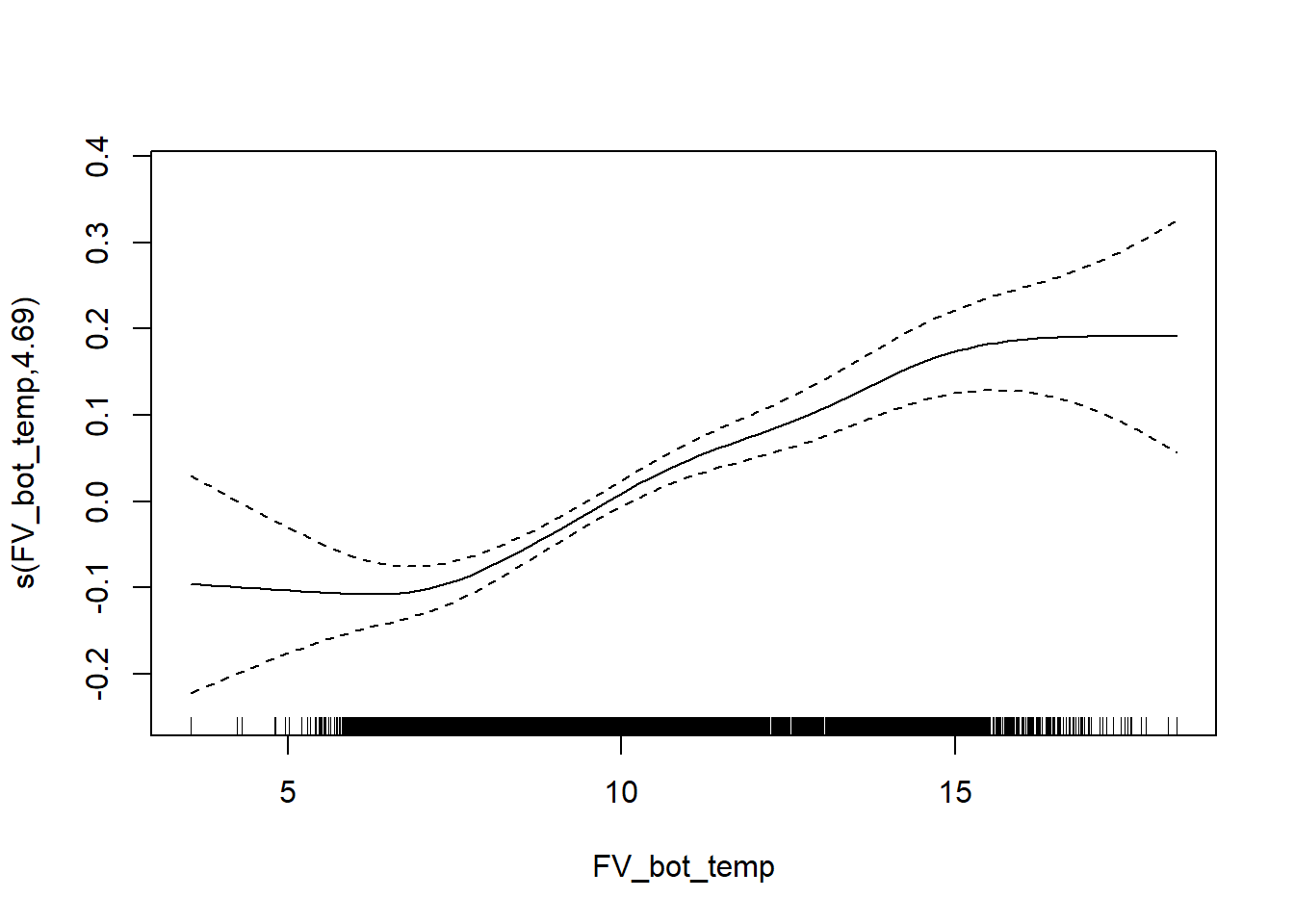
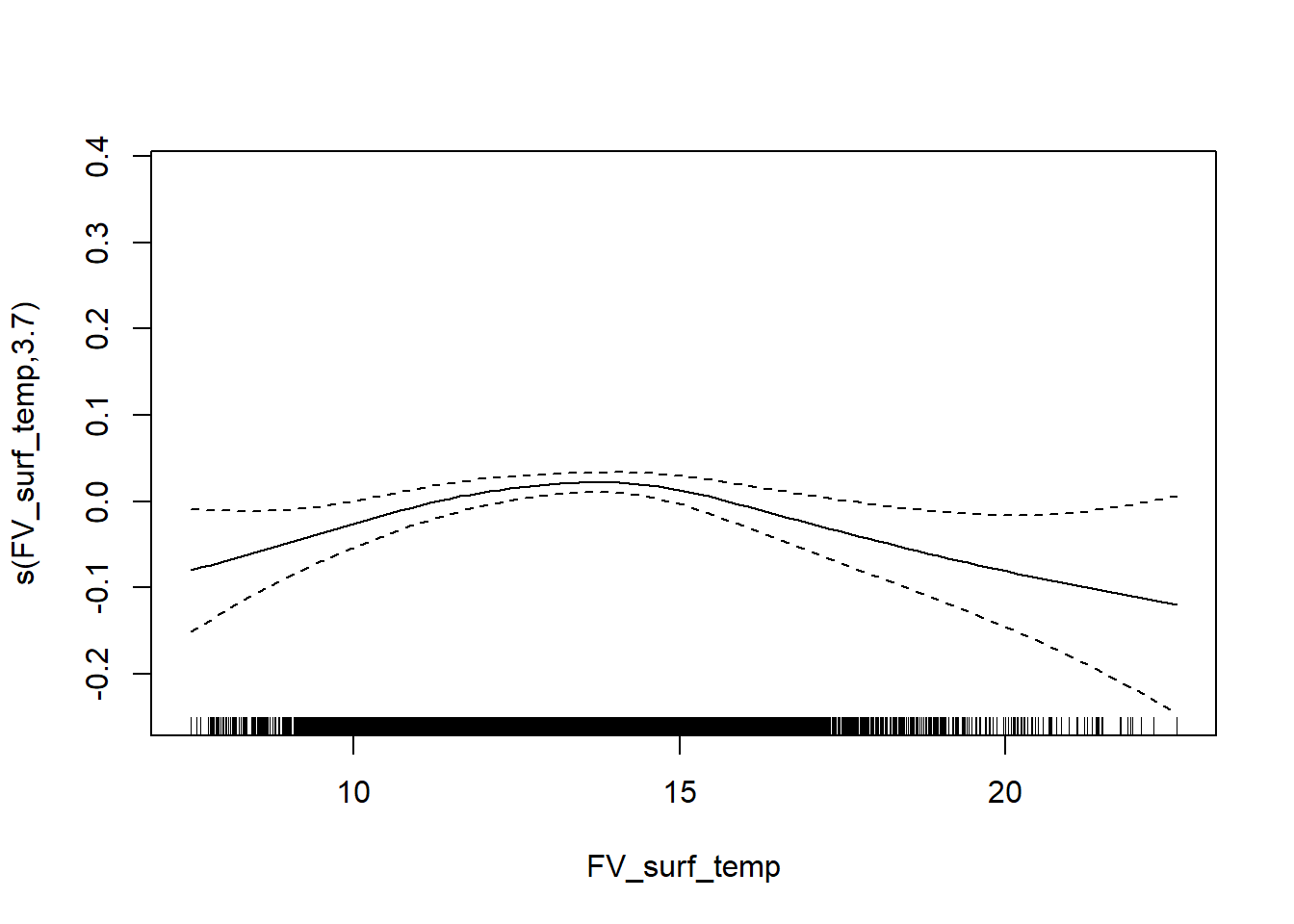
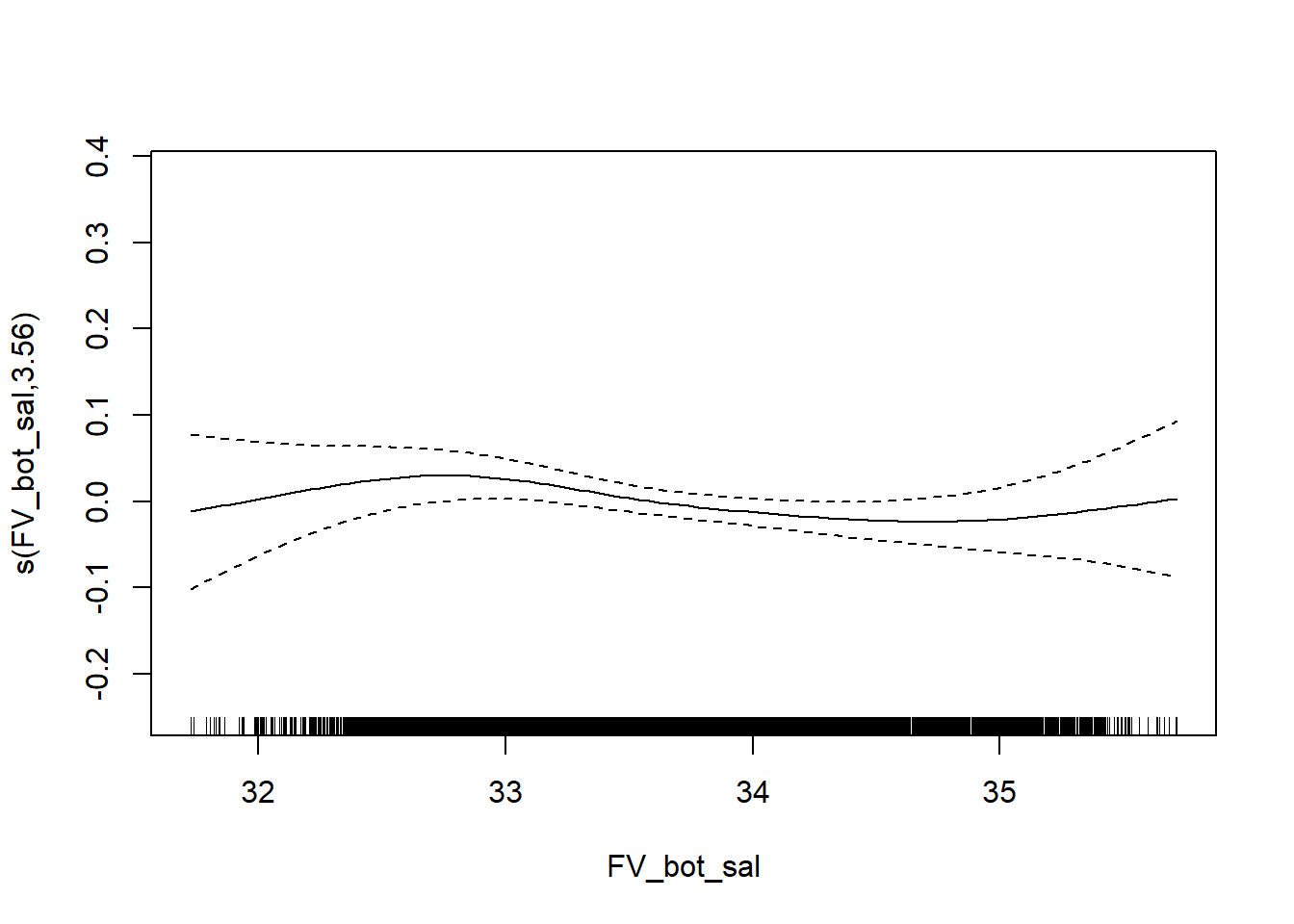
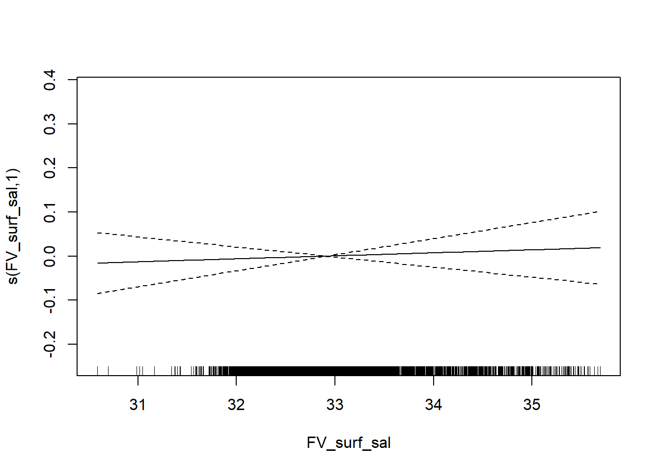
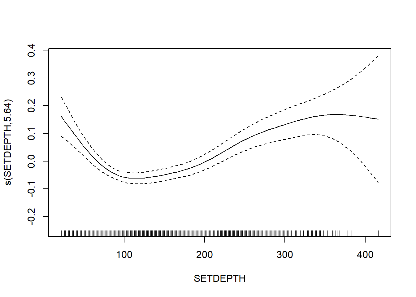
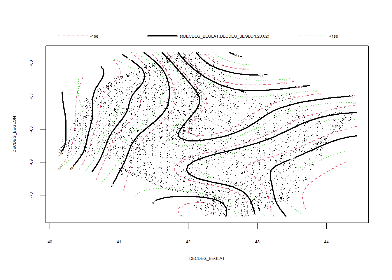
Variation in taxonomic distinctness
FV_GOM_delta_var_FL <- gamm4(delta_var ~ s(FV_bot_temp) + s(FV_surf_temp) + s(FV_bot_sal) +  s(FV_surf_sal) +   s(SETDEPTH)+ s(DECDEG_BEGLAT, DECDEG_BEGLON) , random = ~ (1|EST_YEAR), data = GOM_fall)

gam.check(FV_GOM_delta_var_FL$gam)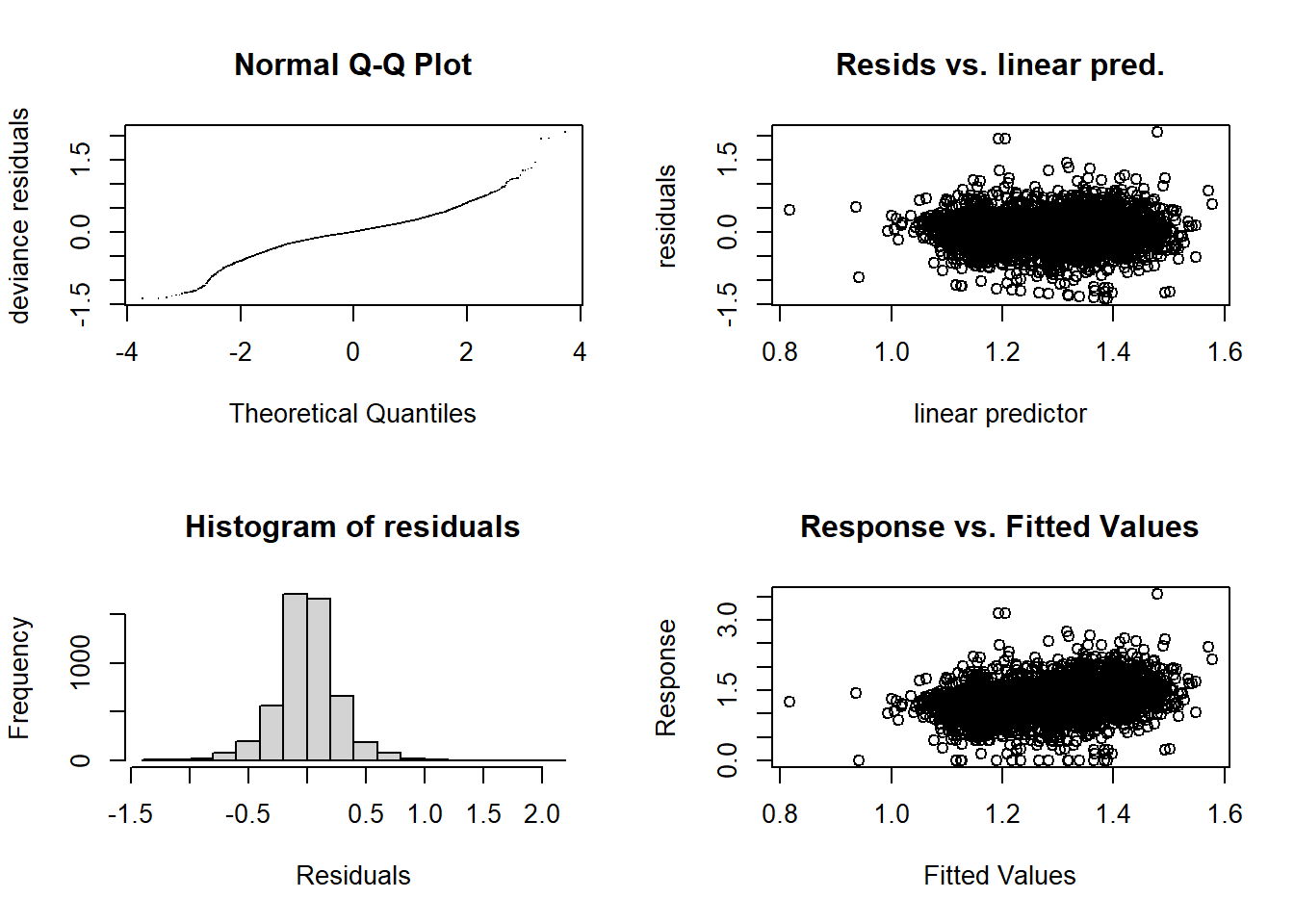
##
## 'gamm' based fit - care required with interpretation.
## Checks based on working residuals may be misleading.
## Basis dimension (k) checking results. Low p-value (k-index<1) may
## indicate that k is too low, especially if edf is close to k'.
##
##                                   k'   edf k-index p-value
## s(FV_bot_temp)                  9.00  7.11    1.00   0.515
## s(FV_surf_temp)                 9.00  4.94    0.99   0.295
## s(FV_bot_sal)                   9.00  1.00    0.99   0.205
## s(FV_surf_sal)                  9.00  1.06    0.98   0.115
## s(SETDEPTH)                     9.00  4.75    0.98   0.085 .
## s(DECDEG_BEGLAT,DECDEG_BEGLON) 29.00 22.47    0.97   0.020 *
## ---
## Signif. codes: 0 '***' 0.001 '**' 0.01 '*' 0.05 '.' 0.1 ' ' 1summary(FV_GOM_delta_var_FL$gam)##
## Family: gaussian
## Link function: identity
##
## Formula:
## delta_var ~ s(FV_bot_temp) + s(FV_surf_temp) + s(FV_bot_sal) +
## s(FV_surf_sal) + s(SETDEPTH) + s(DECDEG_BEGLAT, DECDEG_BEGLON)
##
## Parametric coefficients:
## Estimate Std. Error t value Pr(>|t|)
## (Intercept) 1.26995 0.01051 120.9 <2e-16 ***
## ---
## Signif. codes: 0 '***' 0.001 '**' 0.01 '*' 0.05 '.' 0.1 ' ' 1
##
## Approximate significance of smooth terms:
## edf Ref.df F p-value
## s(FV_bot_temp) 7.105 7.105 1.776 0.1777
## s(FV_surf_temp) 4.936 4.936 3.198 0.0133 *
## s(FV_bot_sal) 1.000 1.000 2.881 0.0897 .
## s(FV_surf_sal) 1.065 1.065 4.965 0.0268 *
## s(SETDEPTH) 4.750 4.750 14.868 <2e-16 ***
## s(DECDEG_BEGLAT,DECDEG_BEGLON) 22.471 22.471 9.611 <2e-16 ***
## ---
## Signif. codes: 0 '***' 0.001 '**' 0.01 '*' 0.05 '.' 0.1 ' ' 1
##
## R-sq.(adj) = 0.122
## lmer.REML = 1538 Scale est. = 0.075284 n = 5215plot(FV_GOM_delta_var_FL$gam)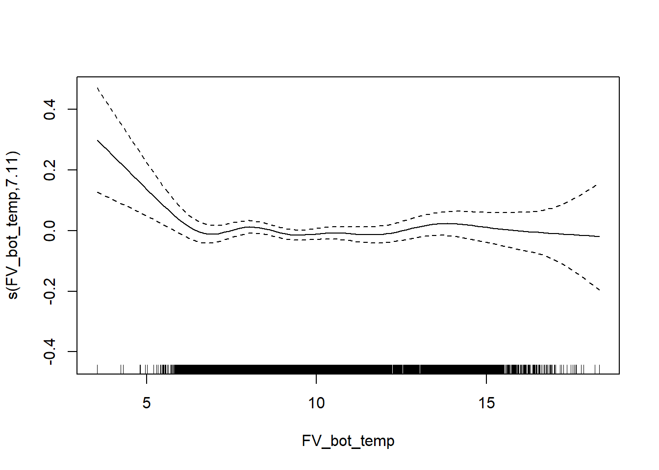
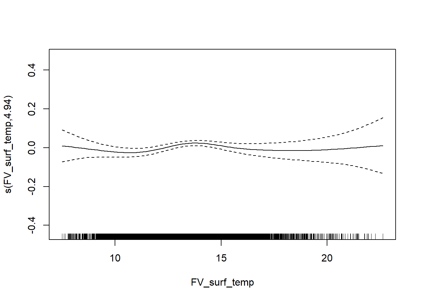
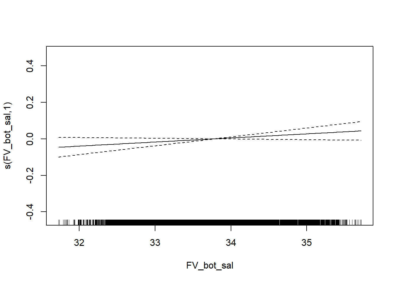
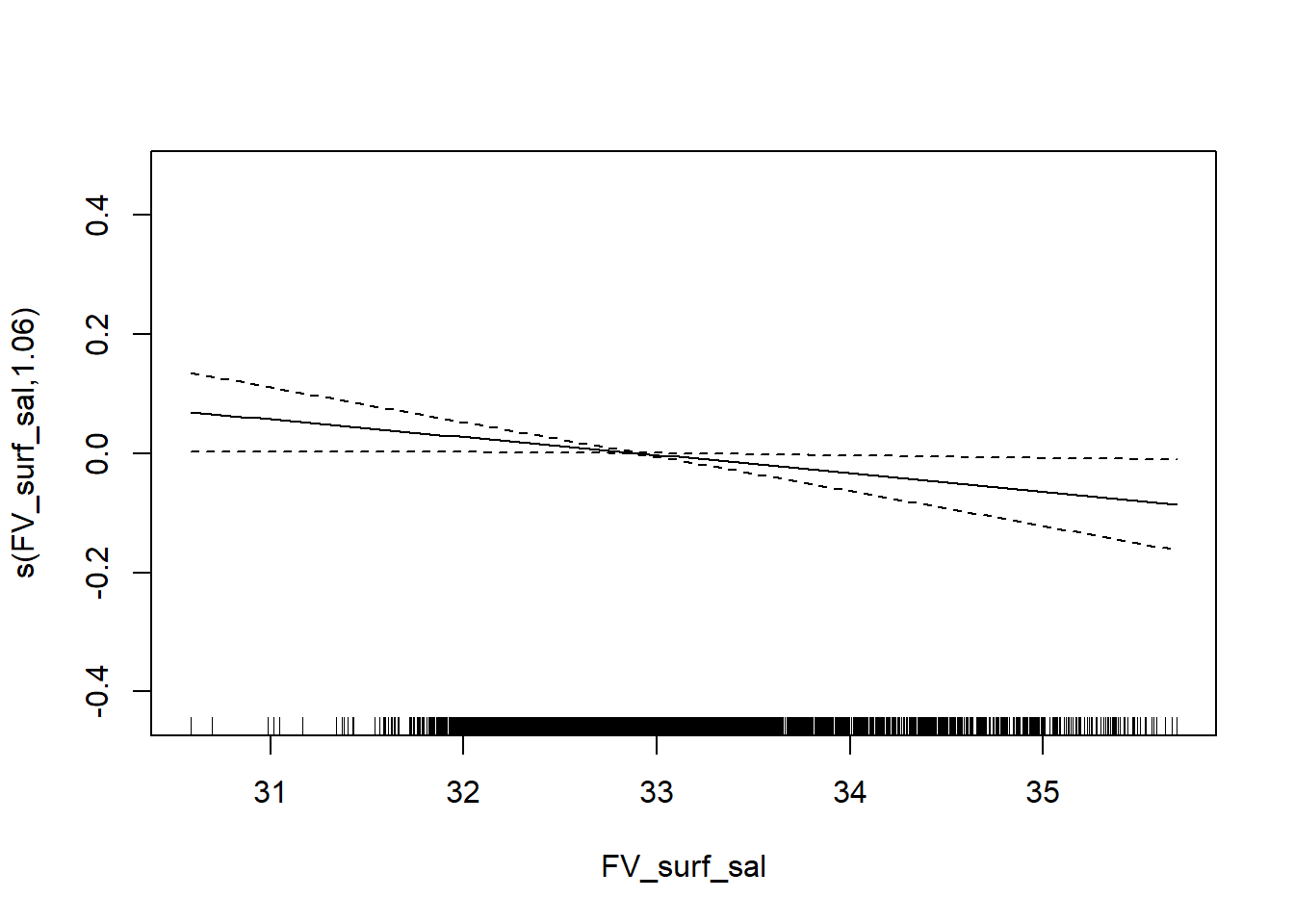
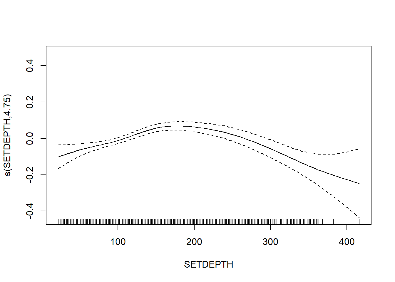
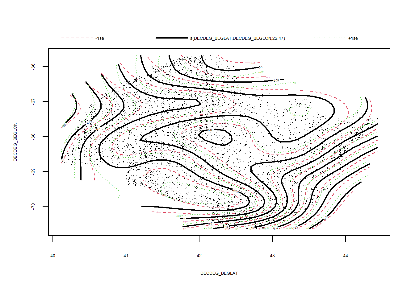
Spring GOM GAMMs
Species richness
FV_GOM_N_SP <- gamm4(N_species ~ s(FV_bot_temp) + s(FV_surf_temp) + s(FV_bot_sal) +  s(FV_surf_sal) + s(SETDEPTH)+ s(DECDEG_BEGLAT, DECDEG_BEGLON) , random = ~ (1|EST_YEAR), data = GOM_spring)

gam.check(FV_GOM_N_SP$gam)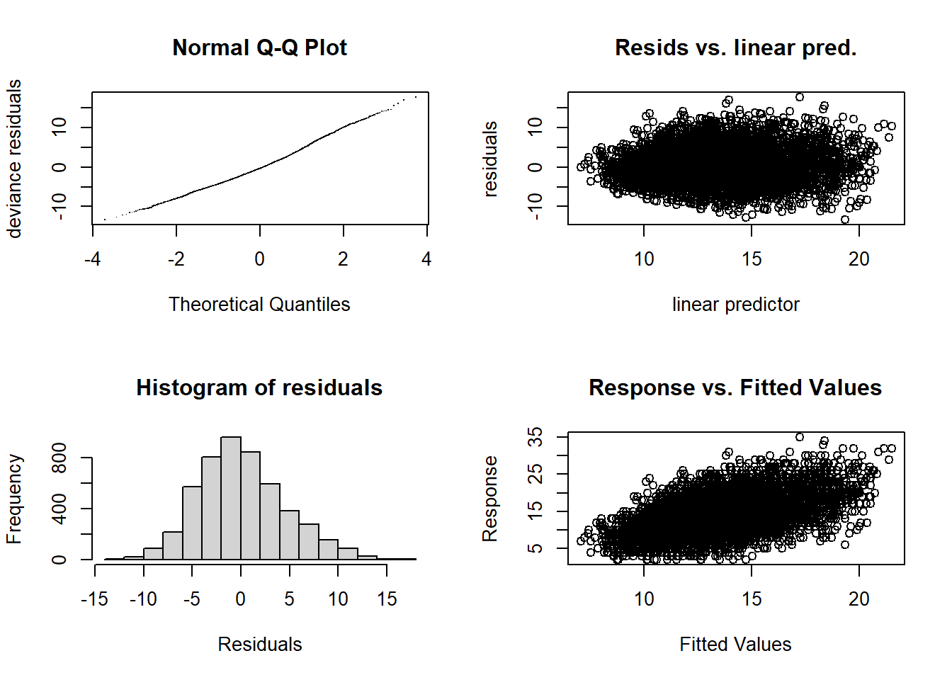
##
## 'gamm' based fit - care required with interpretation.
## Checks based on working residuals may be misleading.
## Basis dimension (k) checking results. Low p-value (k-index<1) may
## indicate that k is too low, especially if edf is close to k'.
##
##                                   k'   edf k-index p-value
## s(FV_bot_temp)                  9.00  3.16    0.95  <2e-16 ***
## s(FV_surf_temp)                 9.00  4.53    0.91  <2e-16 ***
## s(FV_bot_sal)                   9.00  2.61    0.97   0.010 **
## s(FV_surf_sal)                  9.00  5.69    0.97   0.025 *
## s(SETDEPTH)                     9.00  7.10    1.01   0.665
## s(DECDEG_BEGLAT,DECDEG_BEGLON) 29.00 24.64    0.99   0.220
## ---
## Signif. codes: 0 '***' 0.001 '**' 0.01 '*' 0.05 '.' 0.1 ' ' 1summary(FV_GOM_N_SP$gam)##
## Family: gaussian
## Link function: identity
##
## Formula:
## N_species ~ s(FV_bot_temp) + s(FV_surf_temp) + s(FV_bot_sal) +
## s(FV_surf_sal) + s(SETDEPTH) + s(DECDEG_BEGLAT, DECDEG_BEGLON)
##
## Parametric coefficients:
## Estimate Std. Error t value Pr(>|t|)
## (Intercept) 13.4815 0.4656 28.96 <2e-16 ***
## ---
## Signif. codes: 0 '***' 0.001 '**' 0.01 '*' 0.05 '.' 0.1 ' ' 1
##
## Approximate significance of smooth terms:
## edf Ref.df F p-value
## s(FV_bot_temp) 3.164 3.164 10.728 5.94e-07 ***
## s(FV_surf_temp) 4.530 4.530 0.730 0.44759
## s(FV_bot_sal) 2.612 2.612 11.121 3.81e-06 ***
## s(FV_surf_sal) 5.692 5.692 3.063 0.00775 **
## s(SETDEPTH) 7.095 7.095 56.784 < 2e-16 ***
## s(DECDEG_BEGLAT,DECDEG_BEGLON) 24.637 24.637 25.810 < 2e-16 ***
## ---
## Signif. codes: 0 '***' 0.001 '**' 0.01 '*' 0.05 '.' 0.1 ' ' 1
##
## R-sq.(adj) = 0.282
## lmer.REML = 26806 Scale est. = 11.265 n = 5038plot(FV_GOM_N_SP$gam)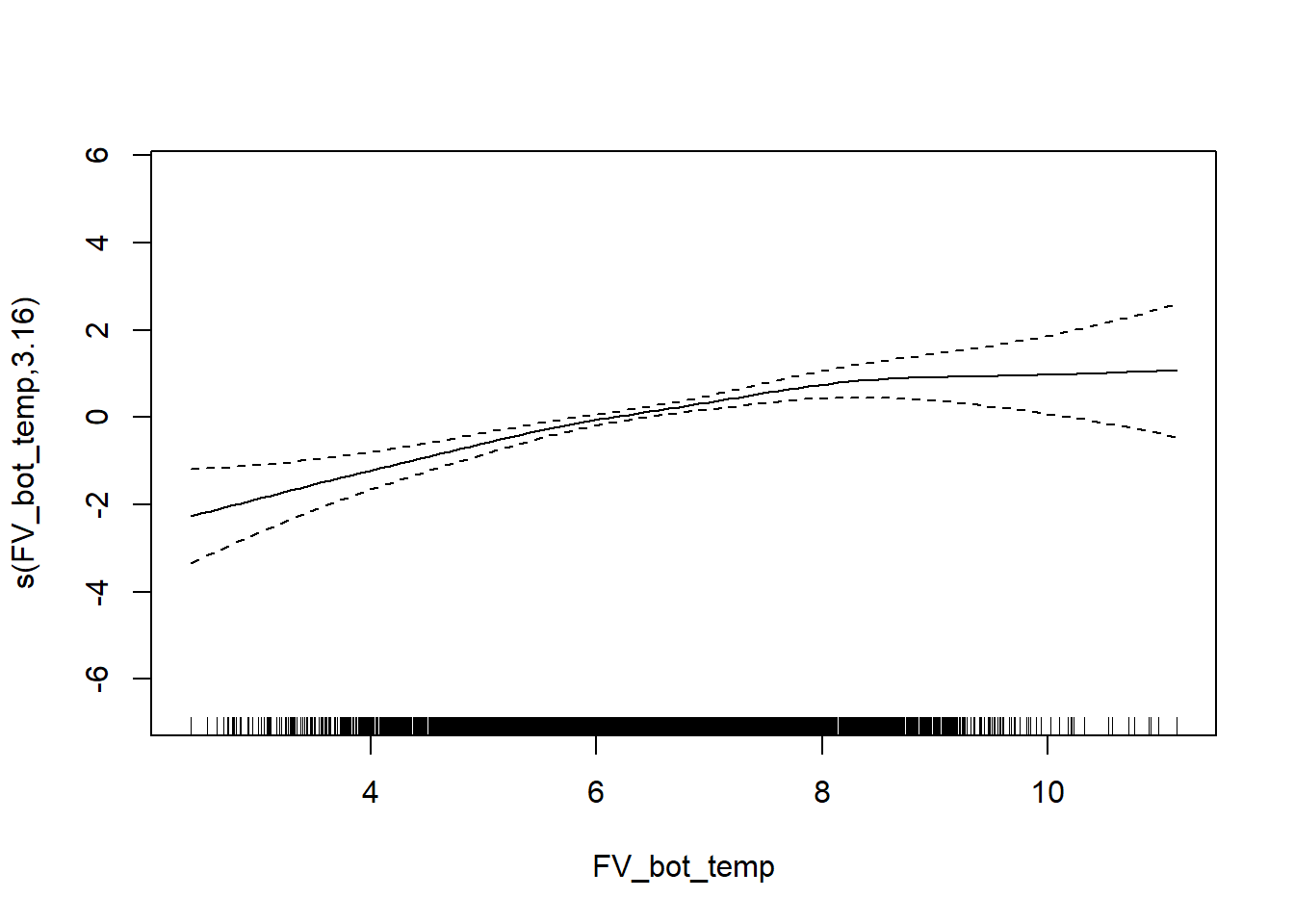
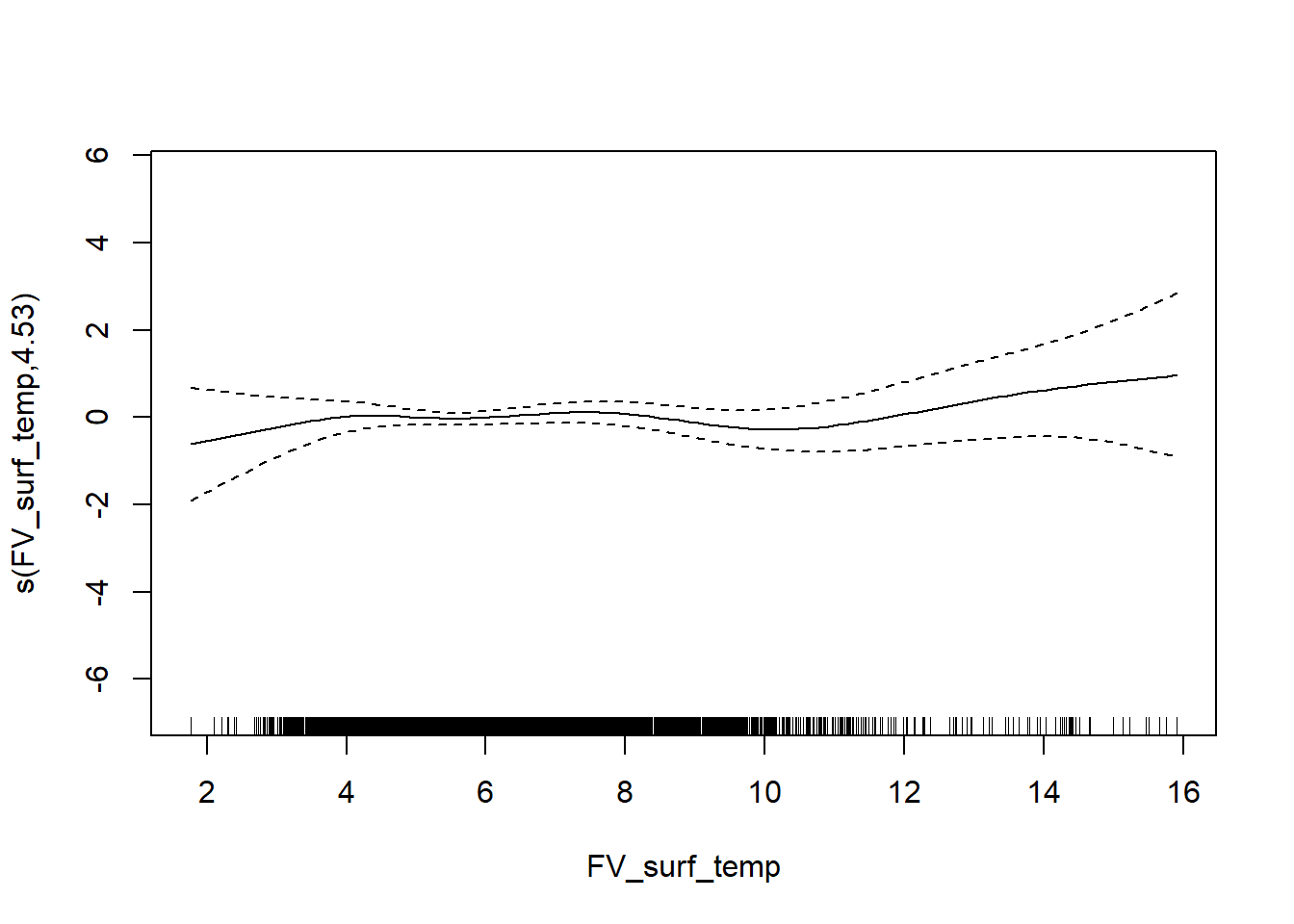
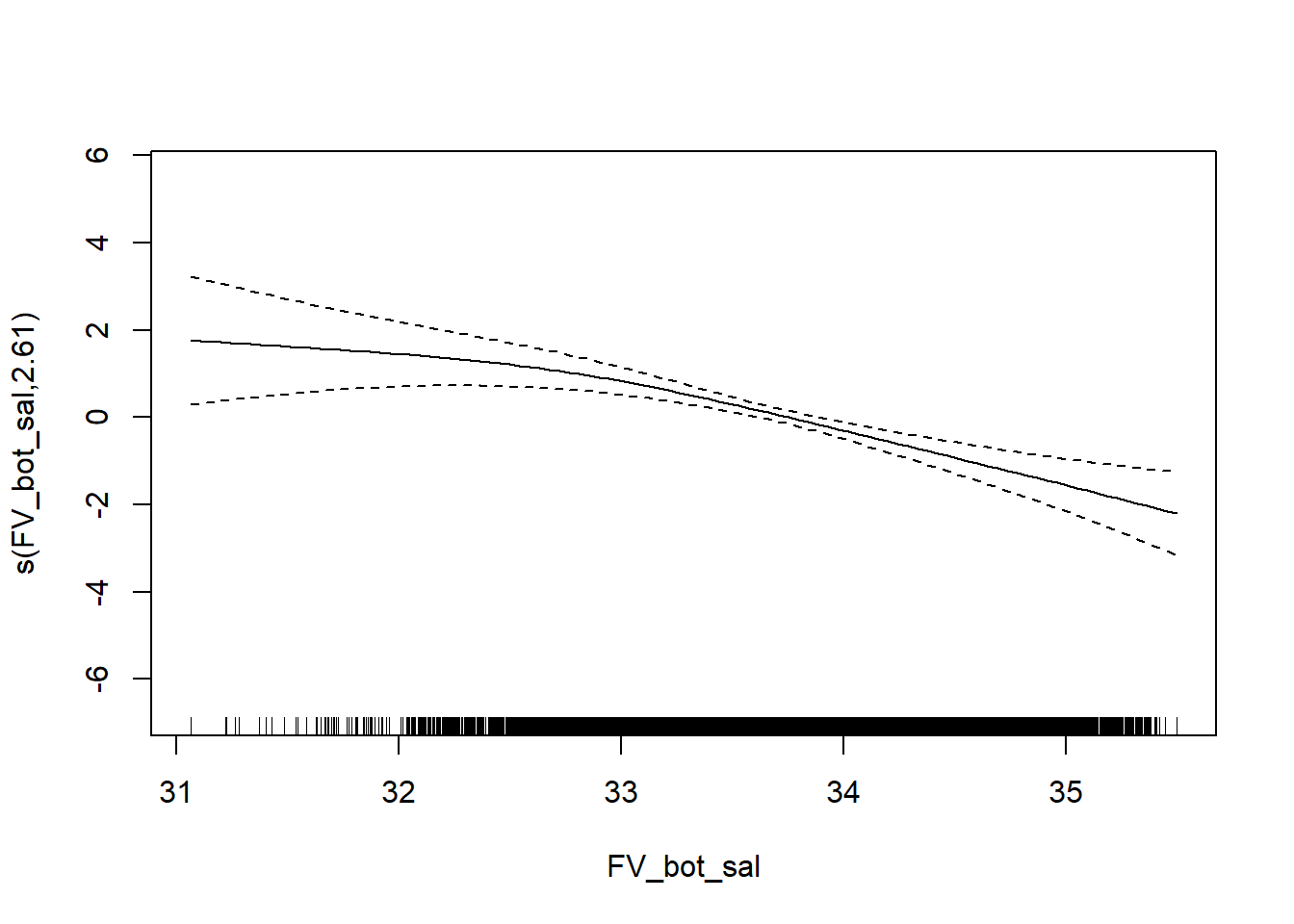
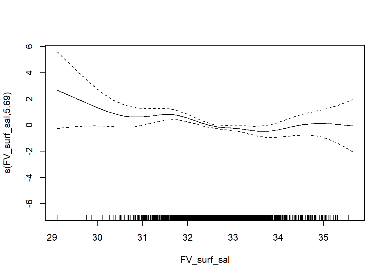
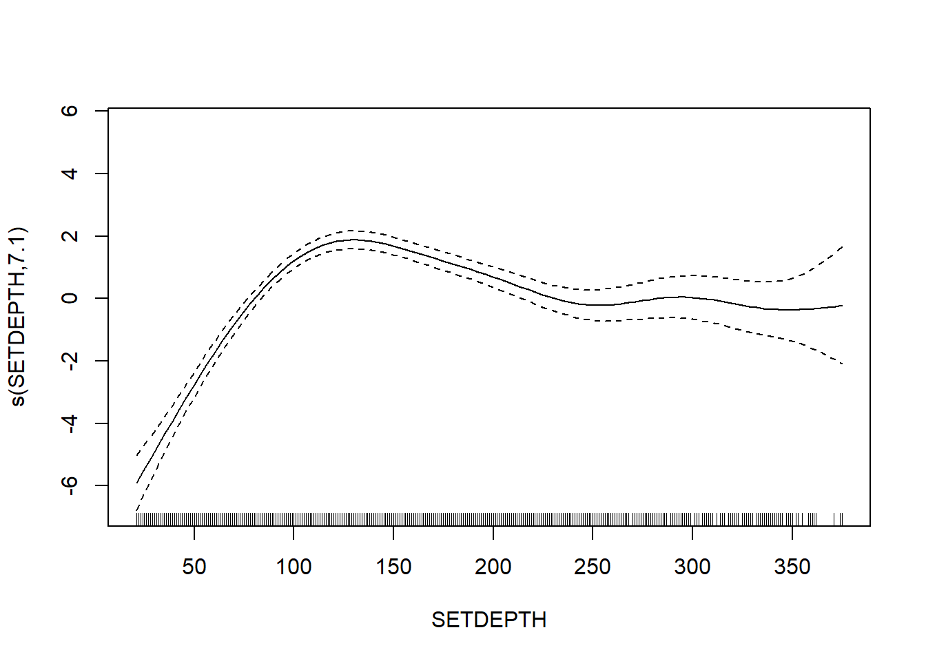
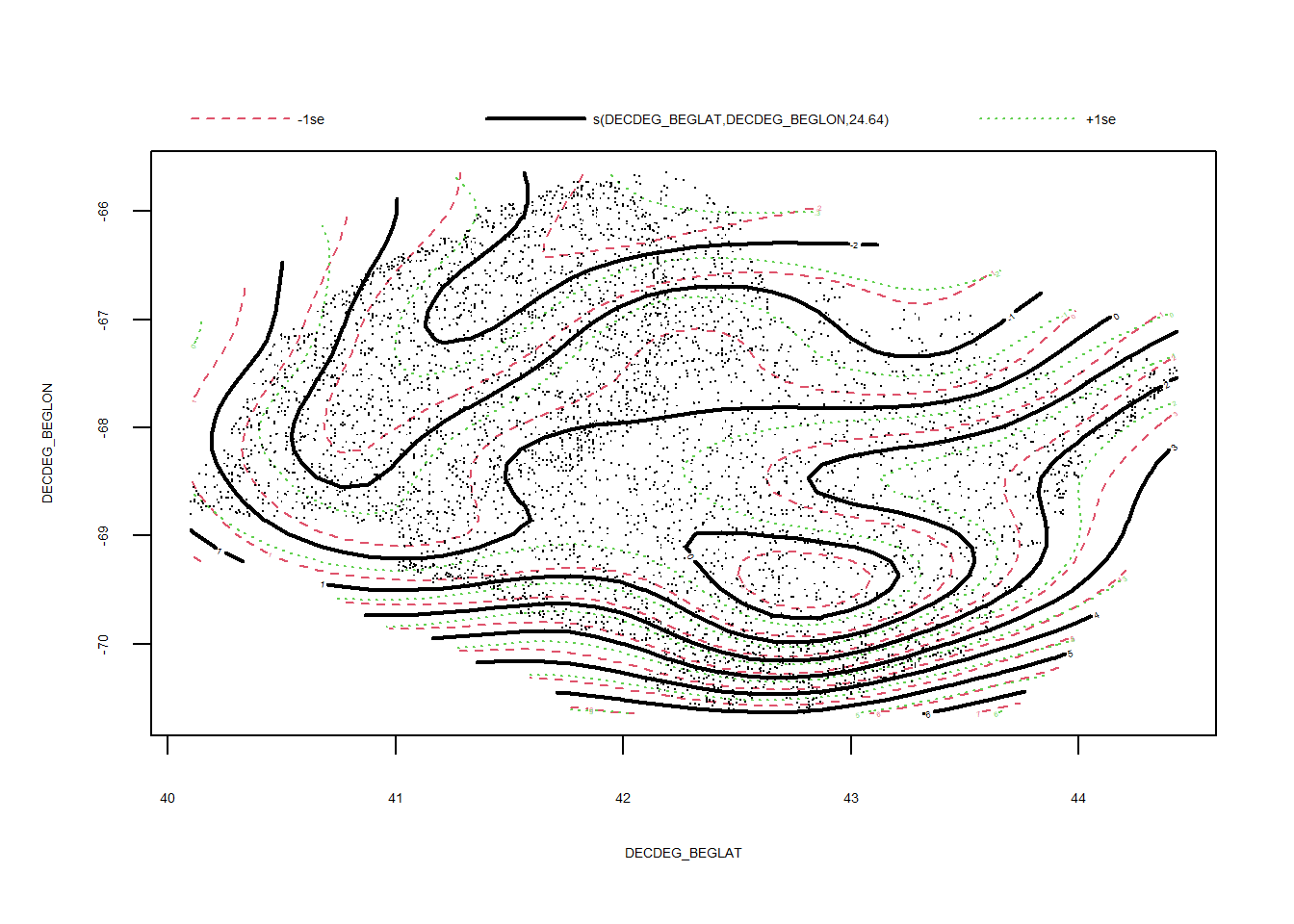
Shannon-Wiener diversity
FV_GOM_H_SP <- gamm4(H_index ~ s(FV_bot_temp) + s(FV_surf_temp) + s(FV_bot_sal) +  s(FV_surf_sal) +  s(SETDEPTH)+ s(DECDEG_BEGLAT, DECDEG_BEGLON) , random = ~ (1|EST_YEAR), data = GOM_spring)

gam.check(FV_GOM_H_SP$gam)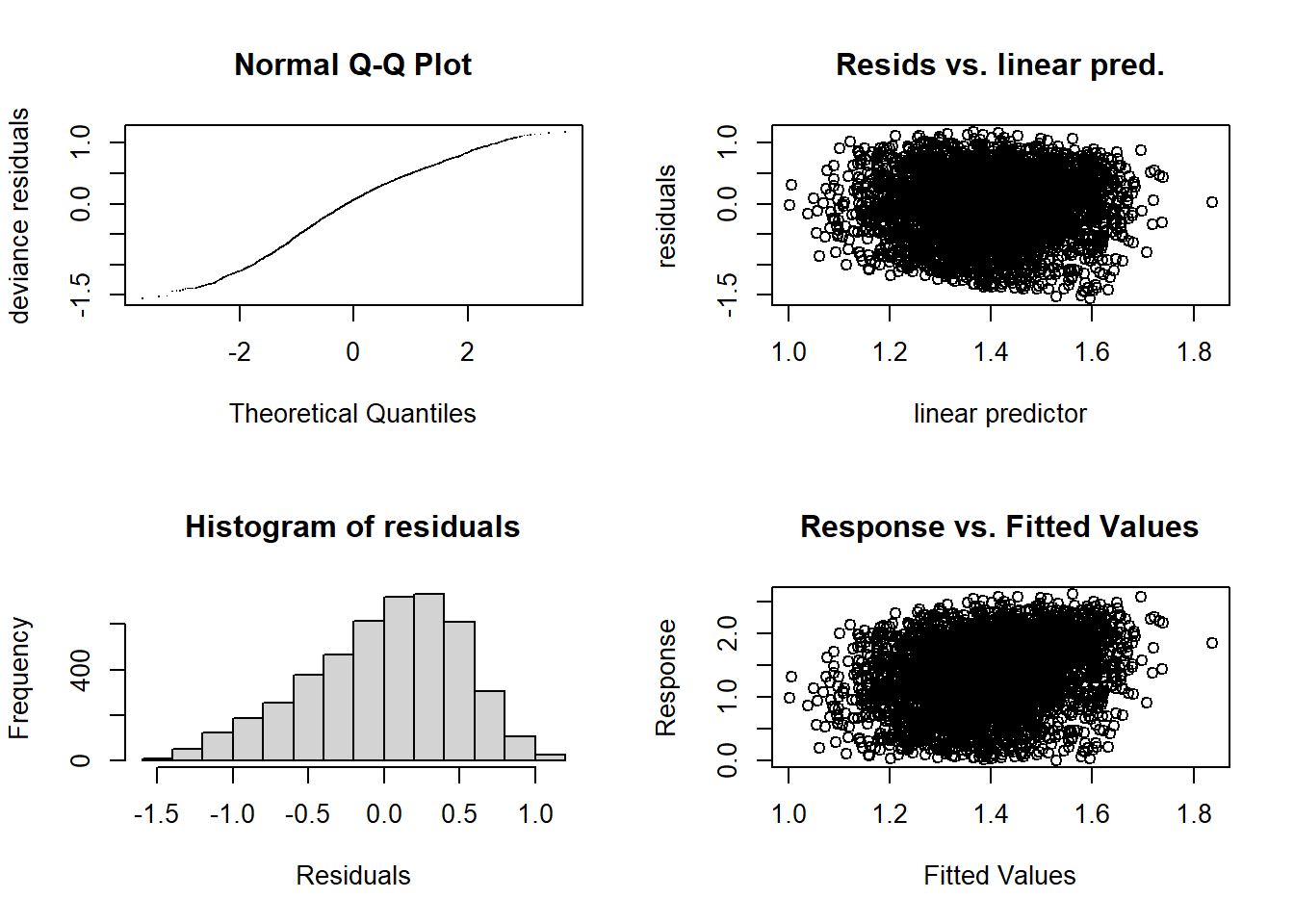
##
## 'gamm' based fit - care required with interpretation.
## Checks based on working residuals may be misleading.
## Basis dimension (k) checking results. Low p-value (k-index<1) may
## indicate that k is too low, especially if edf is close to k'.
##
##                                   k'   edf k-index p-value
## s(FV_bot_temp)                  9.00  3.86    0.99   0.200
## s(FV_surf_temp)                 9.00  3.20    0.99   0.190
## s(FV_bot_sal)                   9.00  1.00    0.97   0.015 *
## s(FV_surf_sal)                  9.00  3.67    1.01   0.780
## s(SETDEPTH)                     9.00  5.72    0.94  <2e-16 ***
## s(DECDEG_BEGLAT,DECDEG_BEGLON) 29.00 17.33    0.97  <2e-16 ***
## ---
## Signif. codes: 0 '***' 0.001 '**' 0.01 '*' 0.05 '.' 0.1 ' ' 1summary(FV_GOM_H_SP$gam)##
## Family: gaussian
## Link function: identity
##
## Formula:
## H_index ~ s(FV_bot_temp) + s(FV_surf_temp) + s(FV_bot_sal) +
## s(FV_surf_sal) + s(SETDEPTH) + s(DECDEG_BEGLAT, DECDEG_BEGLON)
##
## Parametric coefficients:
## Estimate Std. Error t value Pr(>|t|)
## (Intercept) 1.39873 0.01622 86.24 <2e-16 ***
## ---
## Signif. codes: 0 '***' 0.001 '**' 0.01 '*' 0.05 '.' 0.1 ' ' 1
##
## Approximate significance of smooth terms:
## edf Ref.df F p-value
## s(FV_bot_temp) 3.862 3.862 6.687 3.13e-05 ***
## s(FV_surf_temp) 3.203 3.203 5.089 0.001489 **
## s(FV_bot_sal) 1.000 1.000 0.290 0.589965
## s(FV_surf_sal) 3.668 3.668 1.917 0.083133 .
## s(SETDEPTH) 5.724 5.724 4.479 0.000368 ***
## s(DECDEG_BEGLAT,DECDEG_BEGLON) 17.335 17.335 6.100 < 2e-16 ***
## ---
## Signif. codes: 0 '***' 0.001 '**' 0.01 '*' 0.05 '.' 0.1 ' ' 1
##
## R-sq.(adj) = 0.0507
## lmer.REML = 6734 Scale est. = 0.24557 n = 4577plot(FV_GOM_H_SP$gam)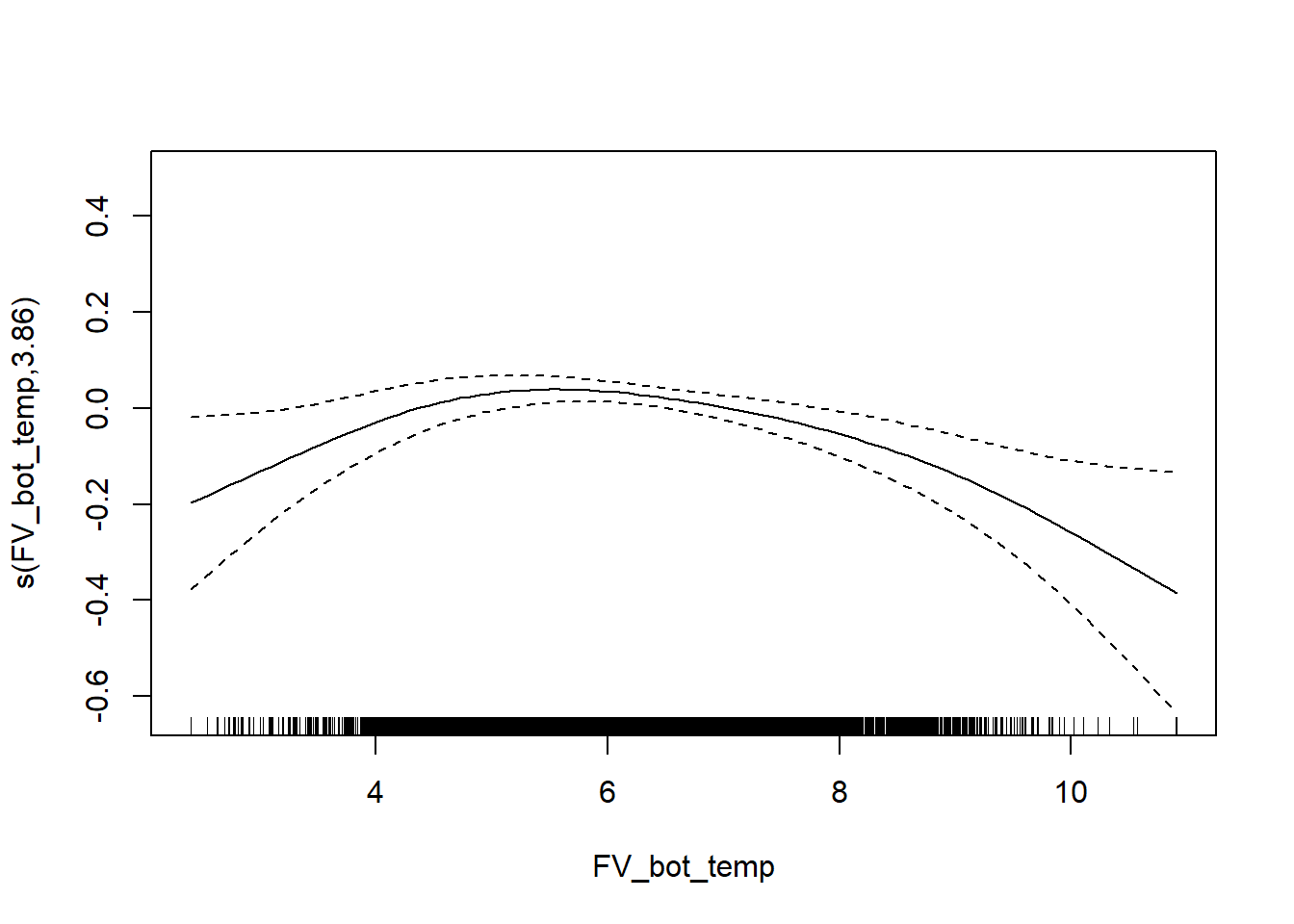
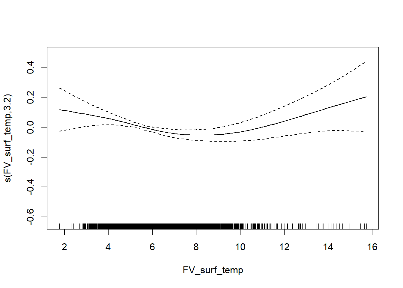
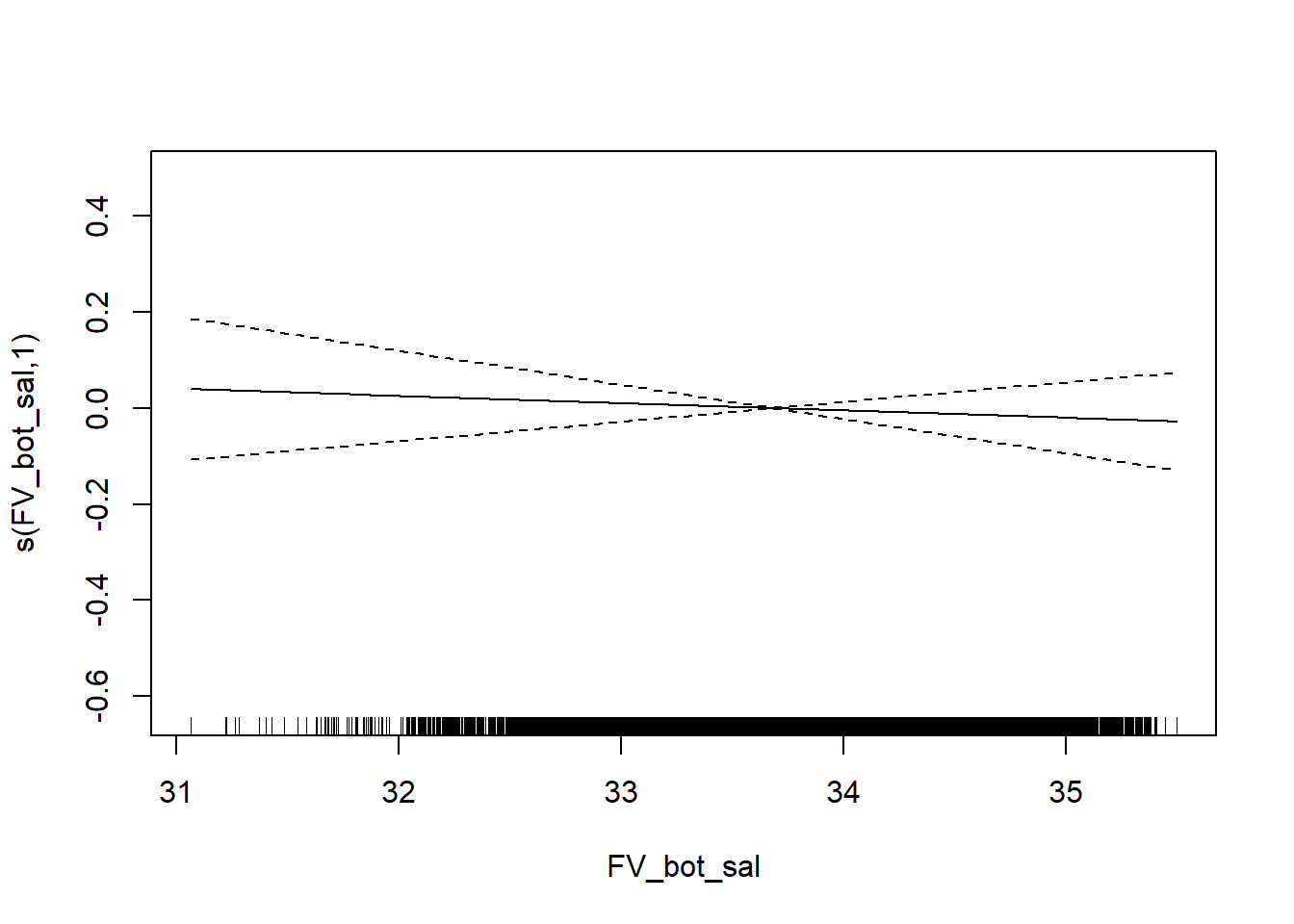
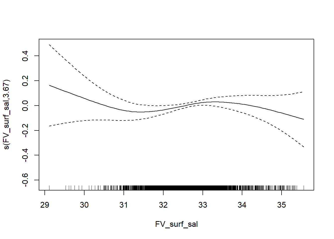
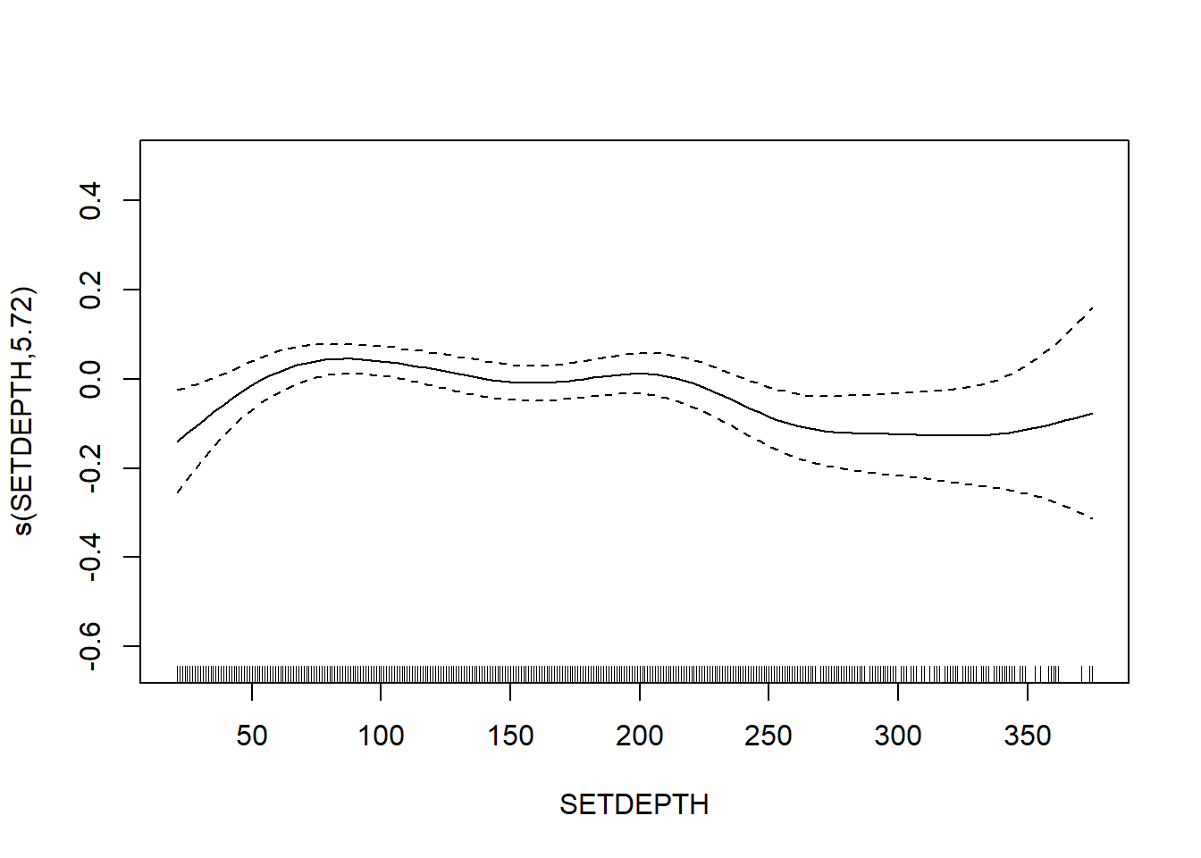
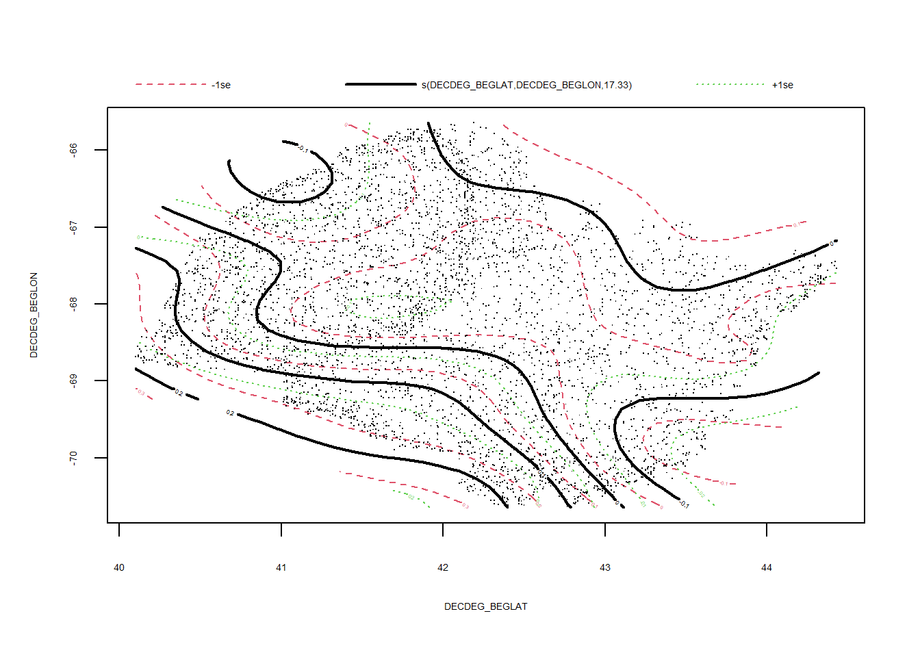
Simpson’s diversity
FV_GOM_D_SP <- gamm4(D_index ~ s(FV_bot_temp) + s(FV_surf_temp) + s(FV_bot_sal) +  s(FV_surf_sal) +   s(SETDEPTH)+ s(DECDEG_BEGLAT, DECDEG_BEGLON) , random = ~ (1|EST_YEAR), data = GOM_spring)

gam.check(FV_GOM_D_SP$gam)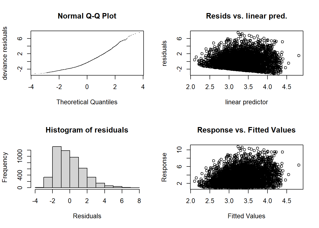
##
## 'gamm' based fit - care required with interpretation.
## Checks based on working residuals may be misleading.
## Basis dimension (k) checking results. Low p-value (k-index<1) may
## indicate that k is too low, especially if edf is close to k'.
##
##                                   k'   edf k-index p-value
## s(FV_bot_temp)                  9.00  3.86    0.99    0.17
## s(FV_surf_temp)                 9.00  3.11    0.99    0.29
## s(FV_bot_sal)                   9.00  1.00    0.98    0.08 .
## s(FV_surf_sal)                  9.00  4.29    1.01    0.80
## s(SETDEPTH)                     9.00  6.22    0.99    0.19
## s(DECDEG_BEGLAT,DECDEG_BEGLON) 29.00 16.71    0.97  <2e-16 ***
## ---
## Signif. codes: 0 '***' 0.001 '**' 0.01 '*' 0.05 '.' 0.1 ' ' 1summary(FV_GOM_D_SP$gam)##
## Family: gaussian
## Link function: identity
##
## Formula:
## D_index ~ s(FV_bot_temp) + s(FV_surf_temp) + s(FV_bot_sal) +
## s(FV_surf_sal) + s(SETDEPTH) + s(DECDEG_BEGLAT, DECDEG_BEGLON)
##
## Parametric coefficients:
## Estimate Std. Error t value Pr(>|t|)
## (Intercept) 3.31363 0.05937 55.81 <2e-16 ***
## ---
## Signif. codes: 0 '***' 0.001 '**' 0.01 '*' 0.05 '.' 0.1 ' ' 1
##
## Approximate significance of smooth terms:
## edf Ref.df F p-value
## s(FV_bot_temp) 3.863 3.863 7.134 1.53e-05 ***
## s(FV_surf_temp) 3.111 3.111 3.772 0.010243 *
## s(FV_bot_sal) 1.000 1.000 0.902 0.342298
## s(FV_surf_sal) 4.290 4.290 2.812 0.025776 *
## s(SETDEPTH) 6.222 6.222 4.272 0.000283 ***
## s(DECDEG_BEGLAT,DECDEG_BEGLON) 16.705 16.705 7.809 < 2e-16 ***
## ---
## Signif. codes: 0 '***' 0.001 '**' 0.01 '*' 0.05 '.' 0.1 ' ' 1
##
## R-sq.(adj) = 0.0596
## lmer.REML = 19330 Scale est. = 2.6261 n = 5038plot(FV_GOM_D_SP$gam)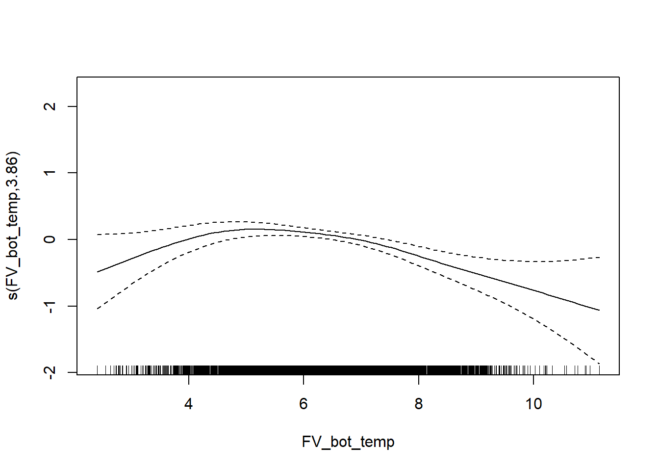
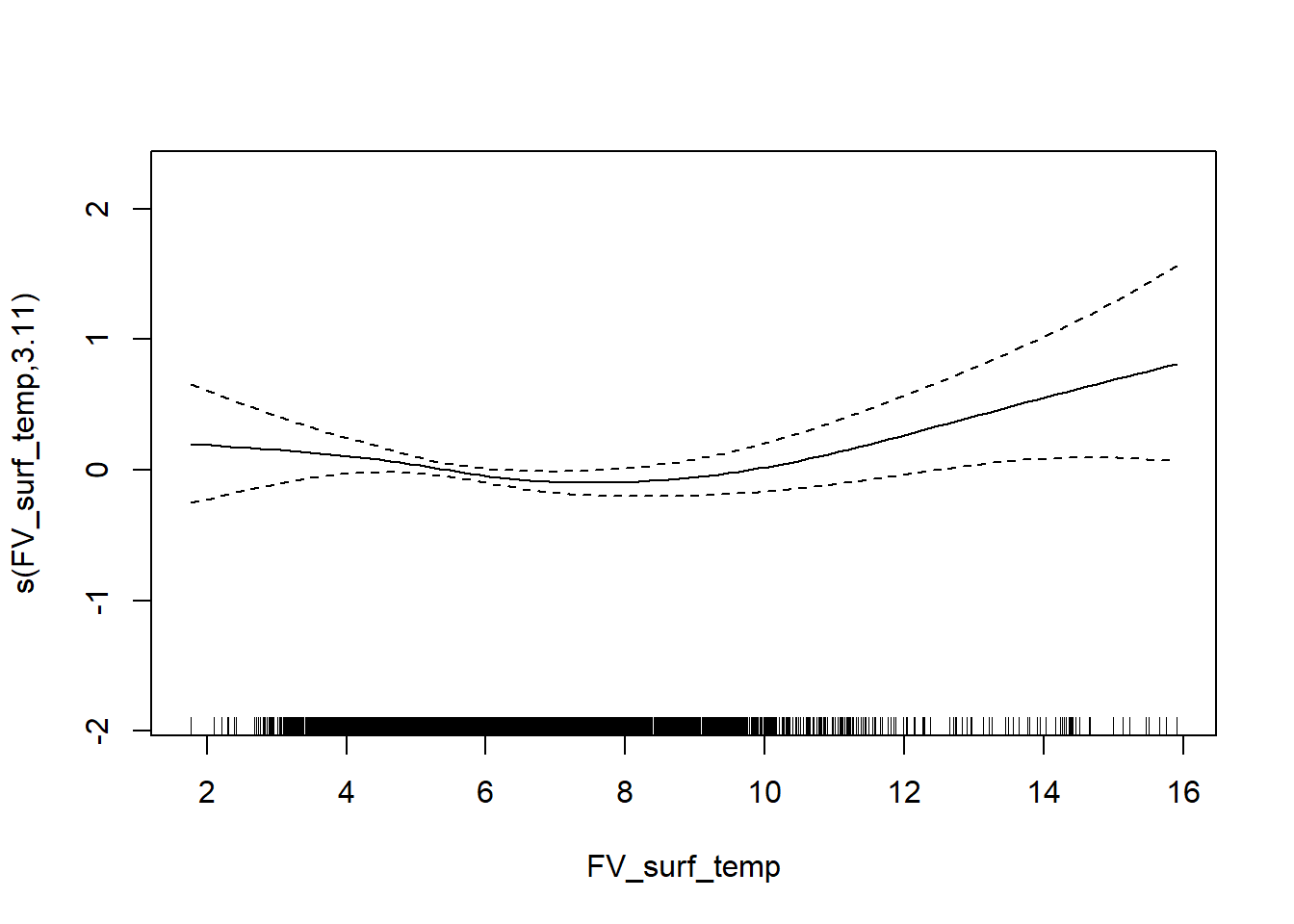
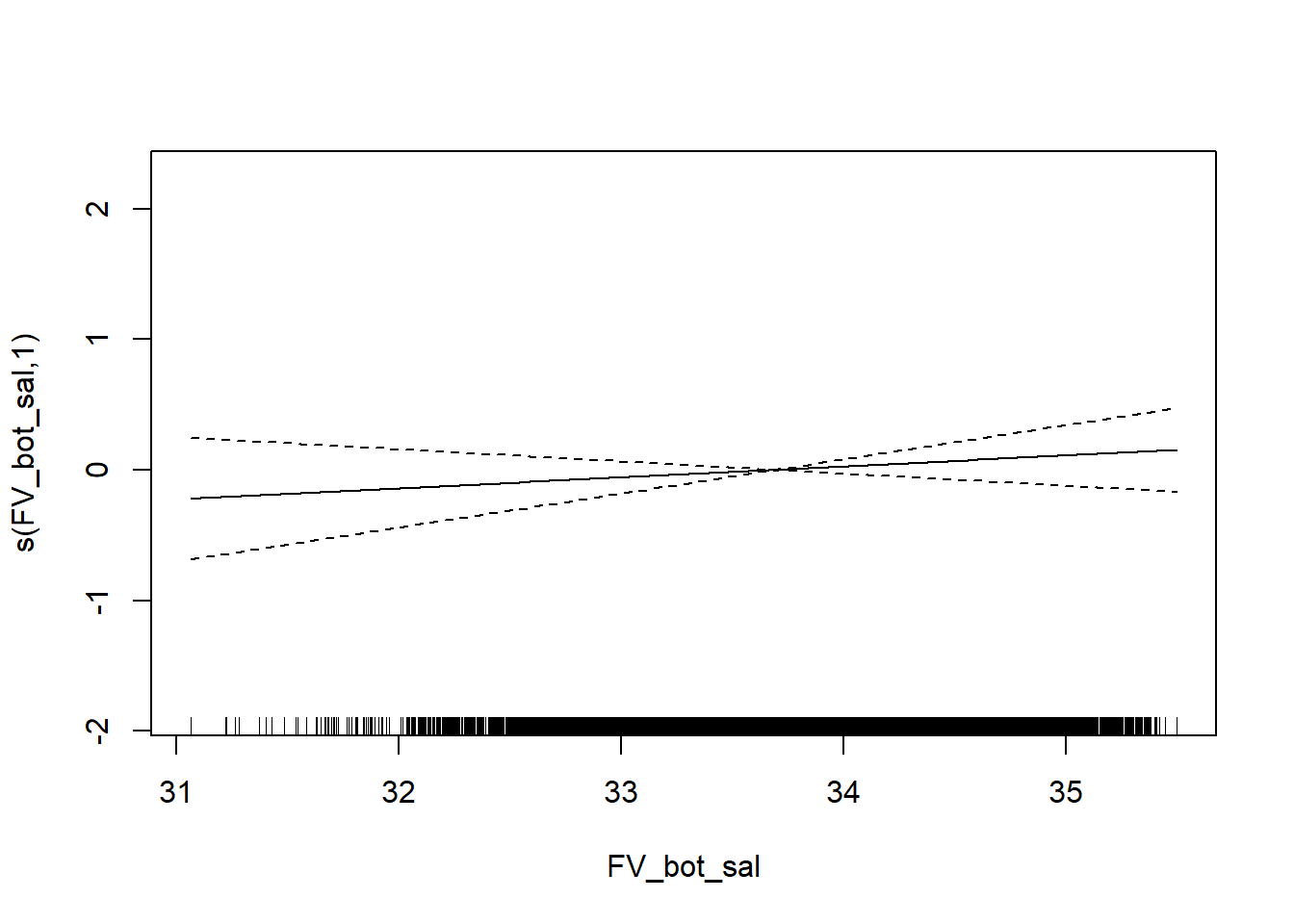
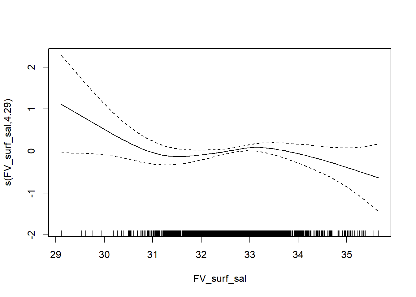
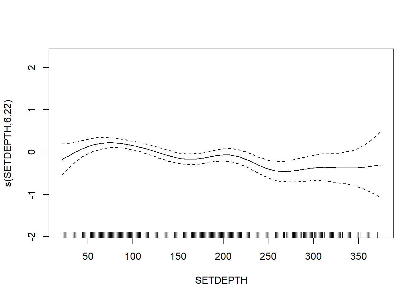
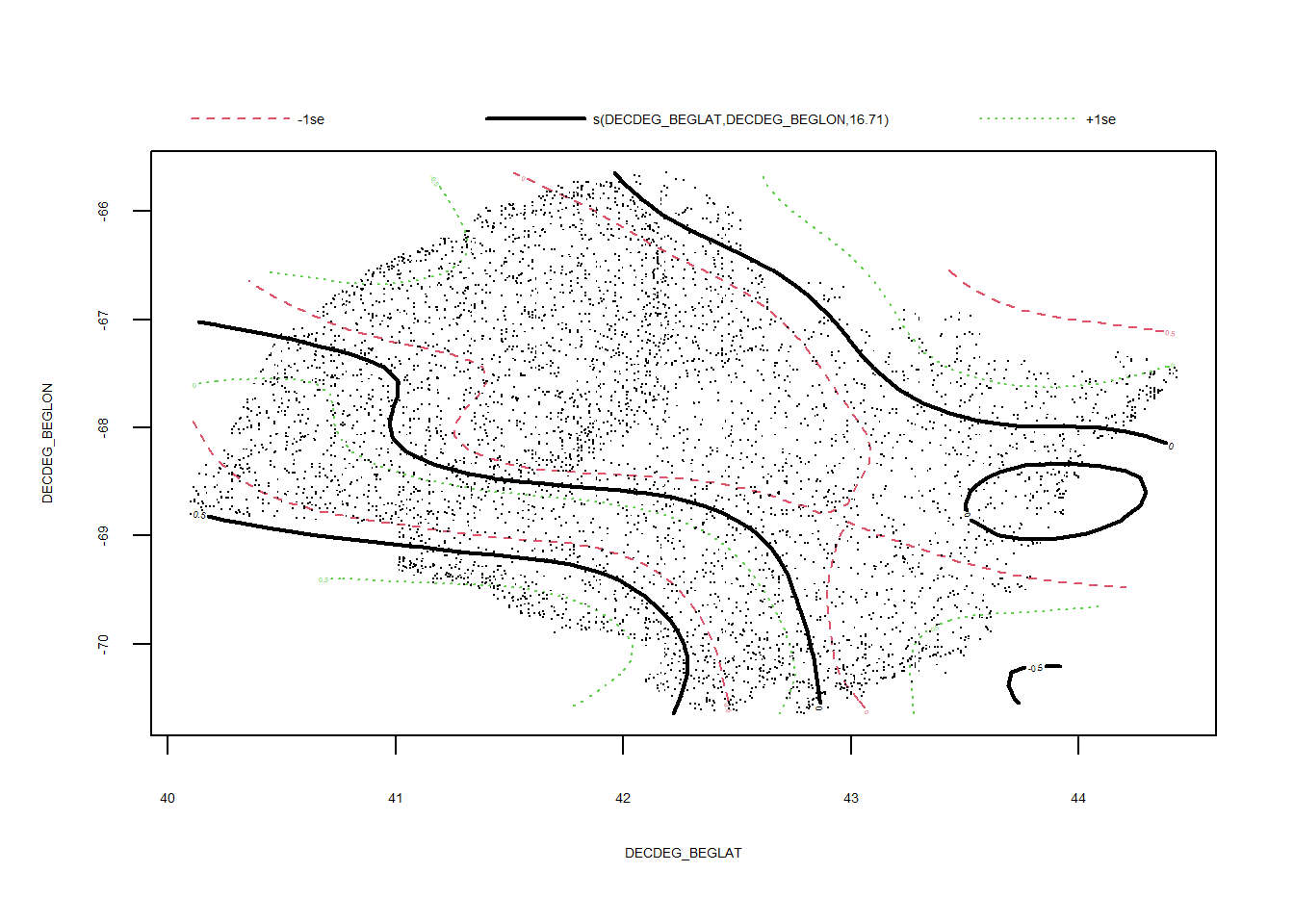
Simpson’s evenness
FV_GOM_E_SP <- gamm4(E_index ~ s(FV_bot_temp) + s(FV_surf_temp) + s(FV_bot_sal) +  s(FV_surf_sal) +  s(SETDEPTH)+ s(DECDEG_BEGLAT, DECDEG_BEGLON) , random = ~ (1|EST_YEAR), data = GOM_spring)

gam.check(FV_GOM_E_SP$gam)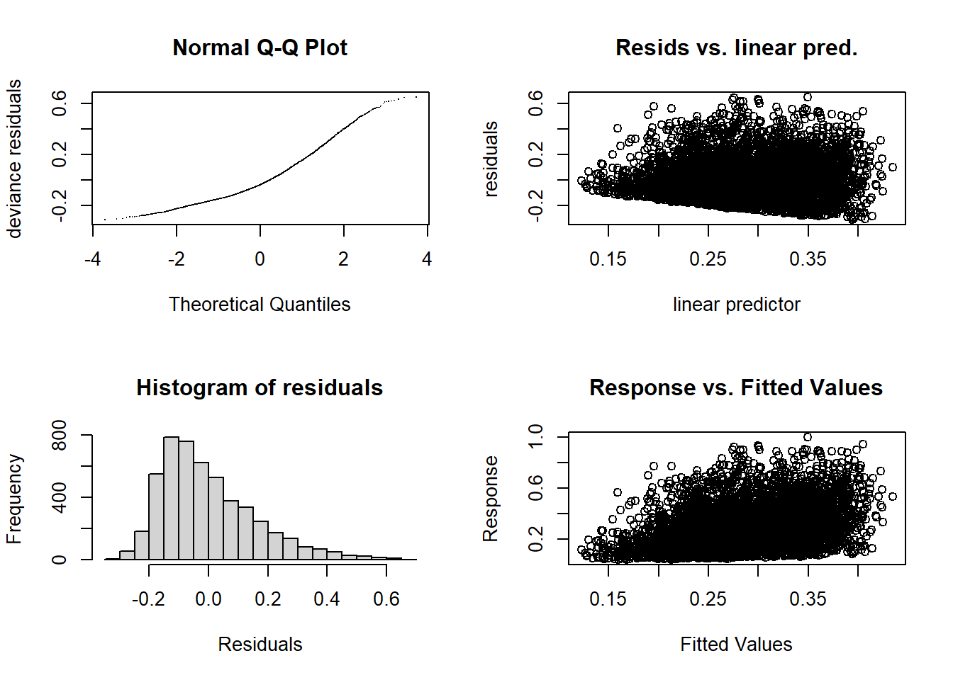
##
## 'gamm' based fit - care required with interpretation.
## Checks based on working residuals may be misleading.
## Basis dimension (k) checking results. Low p-value (k-index<1) may
## indicate that k is too low, especially if edf is close to k'.
##
##                                   k'   edf k-index p-value
## s(FV_bot_temp)                  9.00  4.40    0.99    0.27
## s(FV_surf_temp)                 9.00  2.06    0.97    0.01 **
## s(FV_bot_sal)                   9.00  1.00    1.01    0.76
## s(FV_surf_sal)                  9.00  4.07    0.97    0.03 *
## s(SETDEPTH)                     9.00  5.42    1.03    0.97
## s(DECDEG_BEGLAT,DECDEG_BEGLON) 29.00 22.21    0.96  <2e-16 ***
## ---
## Signif. codes: 0 '***' 0.001 '**' 0.01 '*' 0.05 '.' 0.1 ' ' 1summary(FV_GOM_E_SP$gam)##
## Family: gaussian
## Link function: identity
##
## Formula:
## E_index ~ s(FV_bot_temp) + s(FV_surf_temp) + s(FV_bot_sal) +
## s(FV_surf_sal) + s(SETDEPTH) + s(DECDEG_BEGLAT, DECDEG_BEGLON)
##
## Parametric coefficients:
## Estimate Std. Error t value Pr(>|t|)
## (Intercept) 0.28325 0.01167 24.27 <2e-16 ***
## ---
## Signif. codes: 0 '***' 0.001 '**' 0.01 '*' 0.05 '.' 0.1 ' ' 1
##
## Approximate significance of smooth terms:
## edf Ref.df F p-value
## s(FV_bot_temp) 4.402 4.402 10.463 <2e-16 ***
## s(FV_surf_temp) 2.063 2.063 4.449 0.0124 *
## s(FV_bot_sal) 1.000 1.000 4.303 0.0381 *
## s(FV_surf_sal) 4.070 4.070 2.584 0.0349 *
## s(SETDEPTH) 5.420 5.420 14.604 <2e-16 ***
## s(DECDEG_BEGLAT,DECDEG_BEGLON) 22.212 22.212 9.622 <2e-16 ***
## ---
## Signif. codes: 0 '***' 0.001 '**' 0.01 '*' 0.05 '.' 0.1 ' ' 1
##
## R-sq.(adj) = 0.141
## lmer.REML = -5091.7 Scale est. = 0.020138 n = 5038plot(FV_GOM_E_SP$gam)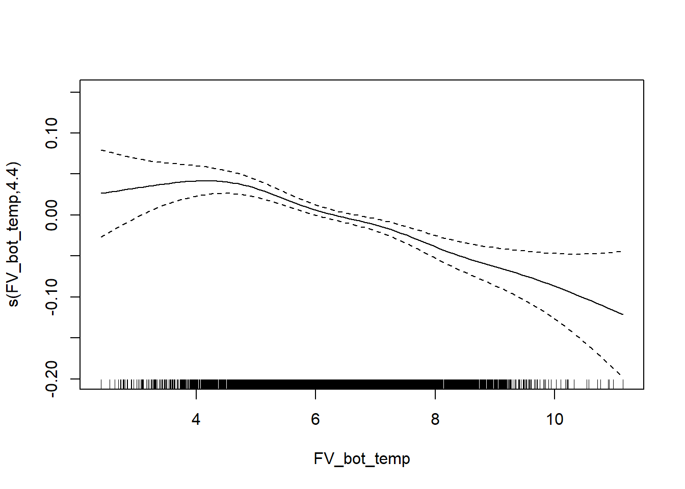
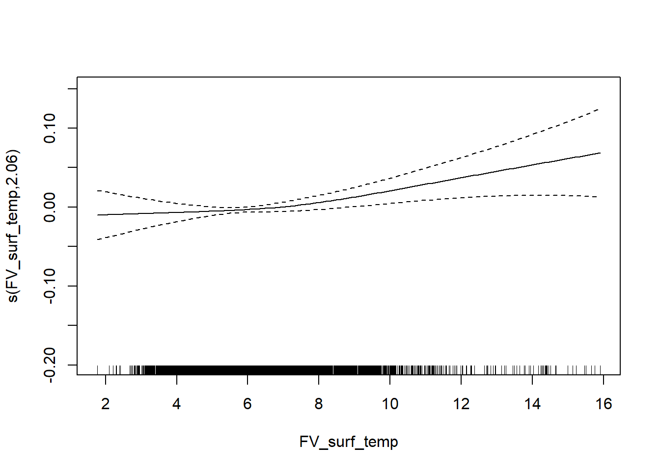
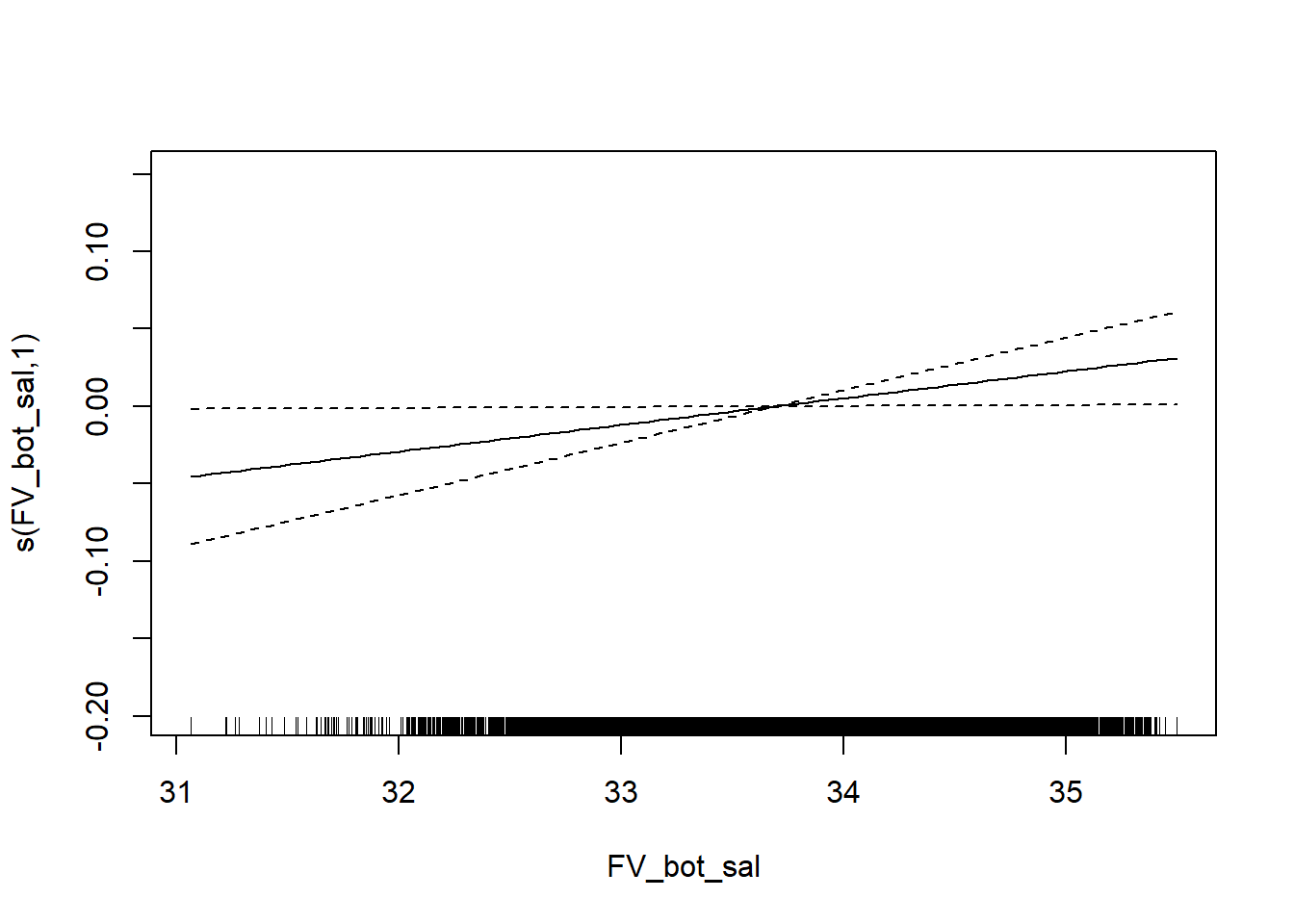
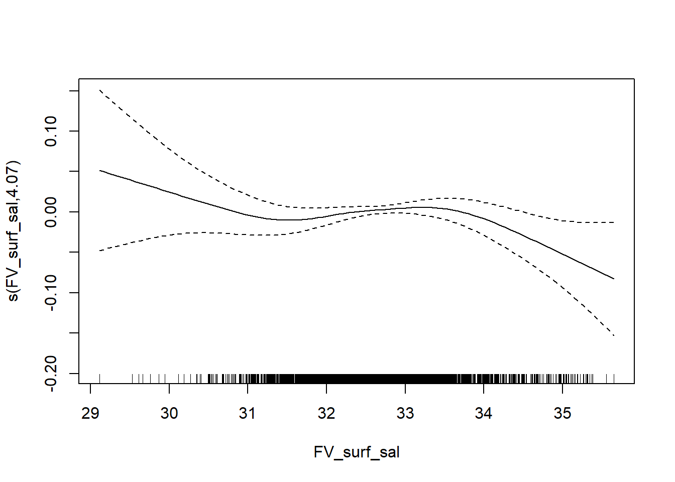
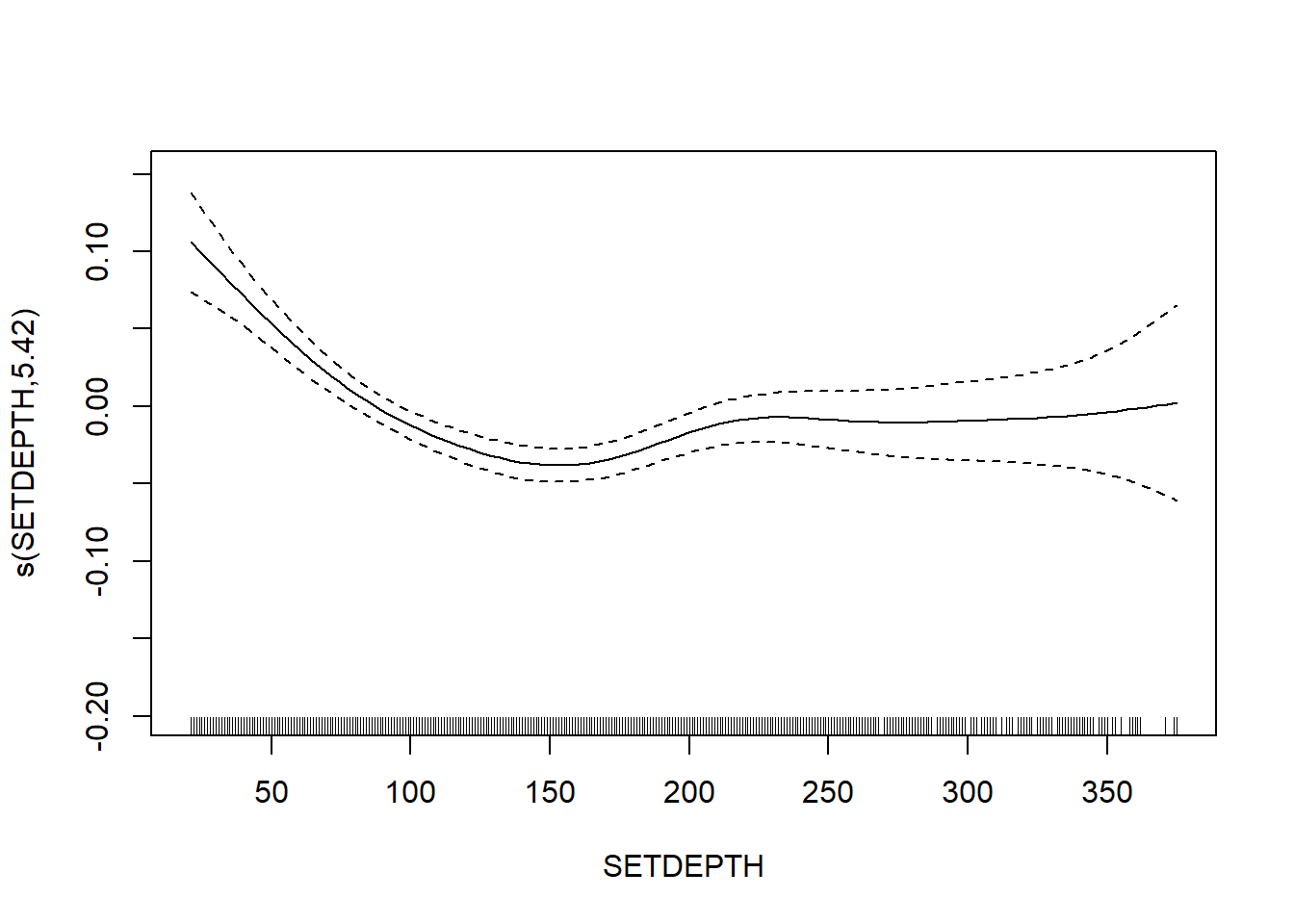
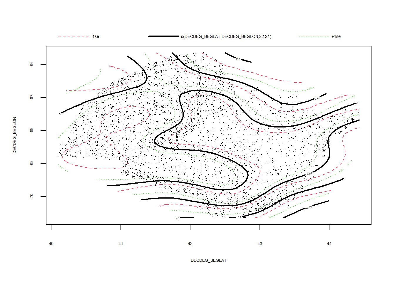
Taxonomic diversity
FV_GOM_delta_SP <- gamm4(delta ~ s(FV_bot_temp) + s(FV_surf_temp) + s(FV_bot_sal) +  s(FV_surf_sal) +  s(SETDEPTH)+ s(DECDEG_BEGLAT, DECDEG_BEGLON) , random = ~ (1|EST_YEAR), data = GOM_spring)

gam.check(FV_GOM_delta_SP$gam)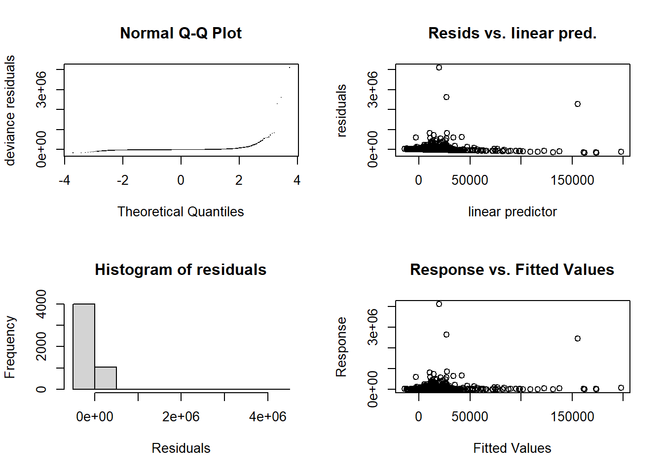
##
## 'gamm' based fit - care required with interpretation.
## Checks based on working residuals may be misleading.
## Basis dimension (k) checking results. Low p-value (k-index<1) may
## indicate that k is too low, especially if edf is close to k'.
##
##                                   k'   edf k-index p-value
## s(FV_bot_temp)                  9.00  3.16    0.95   0.010 **
## s(FV_surf_temp)                 9.00  1.00    1.00   0.315
## s(FV_bot_sal)                   9.00  6.93    1.01   0.995
## s(FV_surf_sal)                  9.00  1.00    1.01   0.915
## s(SETDEPTH)                     9.00  1.00    1.00   0.305
## s(DECDEG_BEGLAT,DECDEG_BEGLON) 29.00  7.77    0.84   0.095 .
## ---
## Signif. codes: 0 '***' 0.001 '**' 0.01 '*' 0.05 '.' 0.1 ' ' 1summary(FV_GOM_delta_SP$gam)##
## Family: gaussian
## Link function: identity
##
## Formula:
## delta ~ s(FV_bot_temp) + s(FV_surf_temp) + s(FV_bot_sal) + s(FV_surf_sal) +
## s(SETDEPTH) + s(DECDEG_BEGLAT, DECDEG_BEGLON)
##
## Parametric coefficients:
## Estimate Std. Error t value Pr(>|t|)
## (Intercept) 11712 3042 3.85 0.00012 ***
## ---
## Signif. codes: 0 '***' 0.001 '**' 0.01 '*' 0.05 '.' 0.1 ' ' 1
##
## Approximate significance of smooth terms:
## edf Ref.df F p-value
## s(FV_bot_temp) 3.162 3.162 1.997 0.0830 .
## s(FV_surf_temp) 1.000 1.000 0.243 0.6218
## s(FV_bot_sal) 6.928 6.928 7.556 <2e-16 ***
## s(FV_surf_sal) 1.000 1.000 0.708 0.4001
## s(SETDEPTH) 1.000 1.000 1.365 0.2427
## s(DECDEG_BEGLAT,DECDEG_BEGLON) 7.767 7.767 1.958 0.0604 .
## ---
## Signif. codes: 0 '***' 0.001 '**' 0.01 '*' 0.05 '.' 0.1 ' ' 1
##
## R-sq.(adj) = 0.0148
## lmer.REML = 1.286e+05 Scale est. = 7.1955e+09 n = 5038plot(FV_GOM_delta_SP$gam)
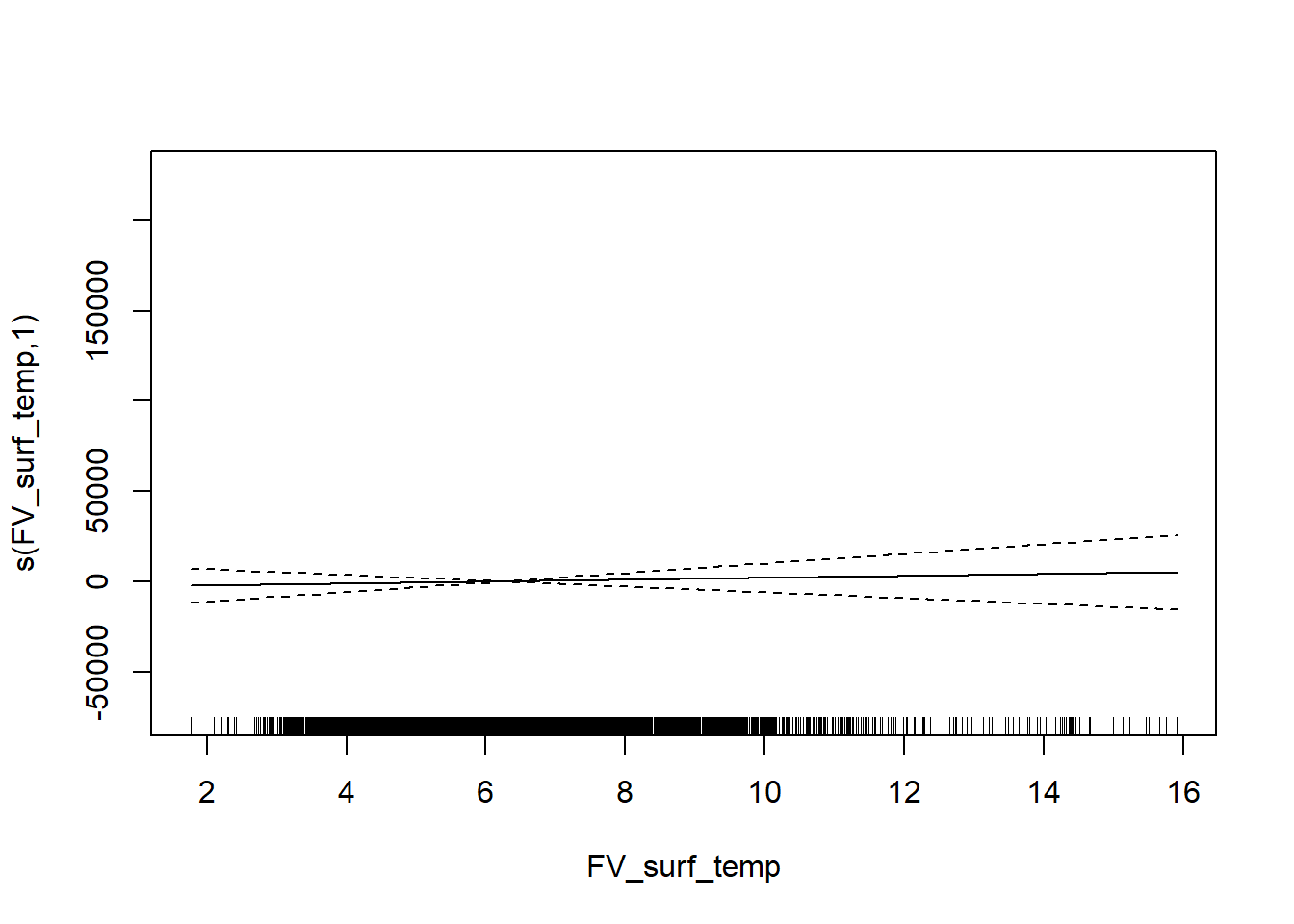
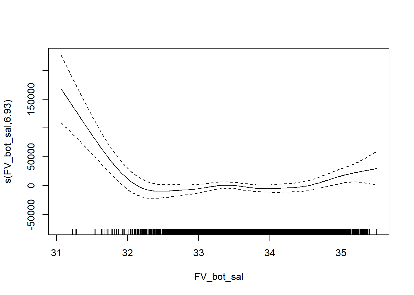
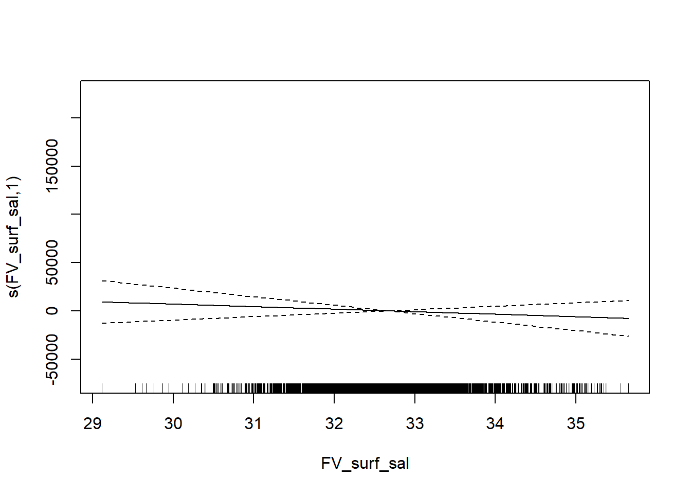
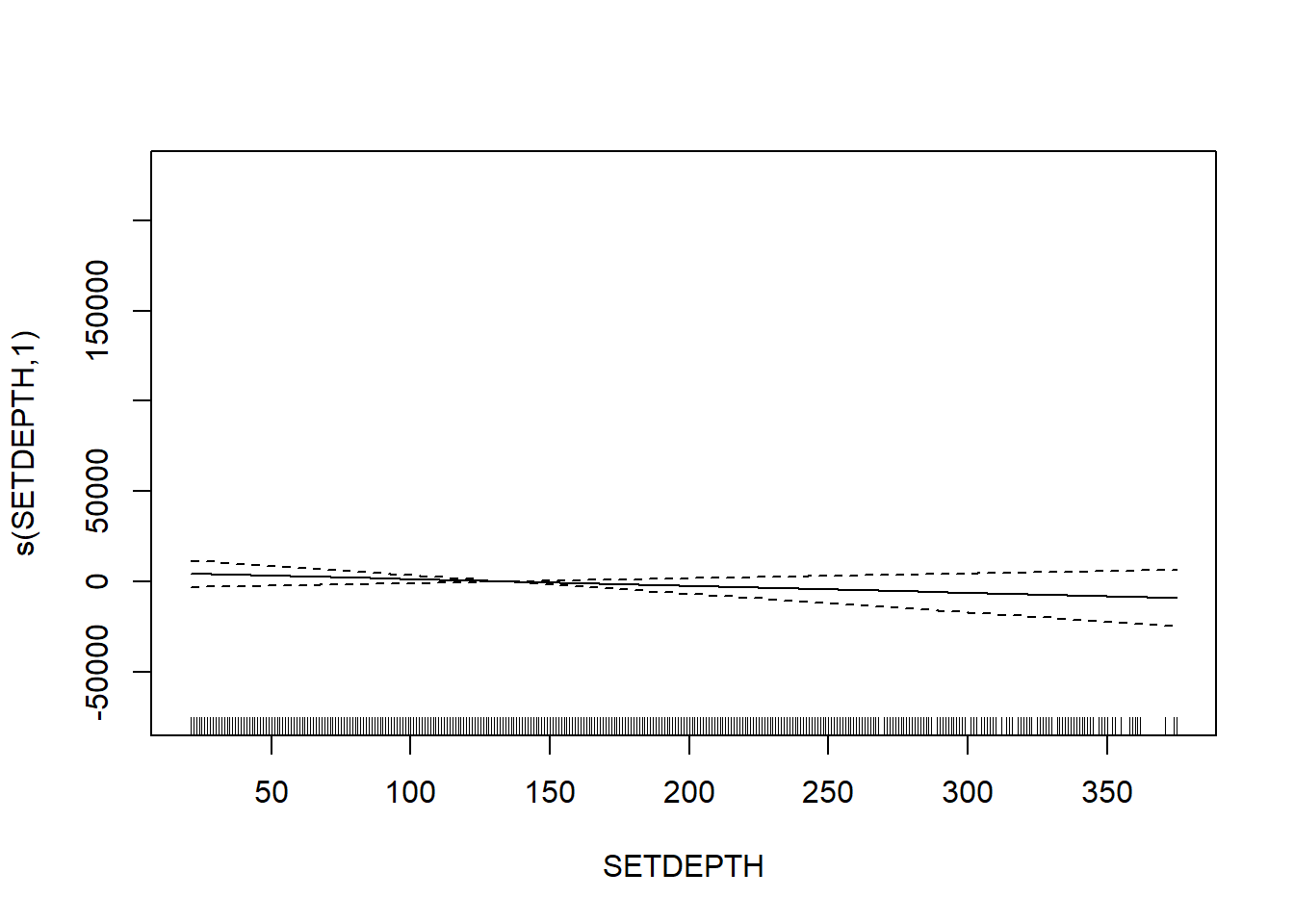
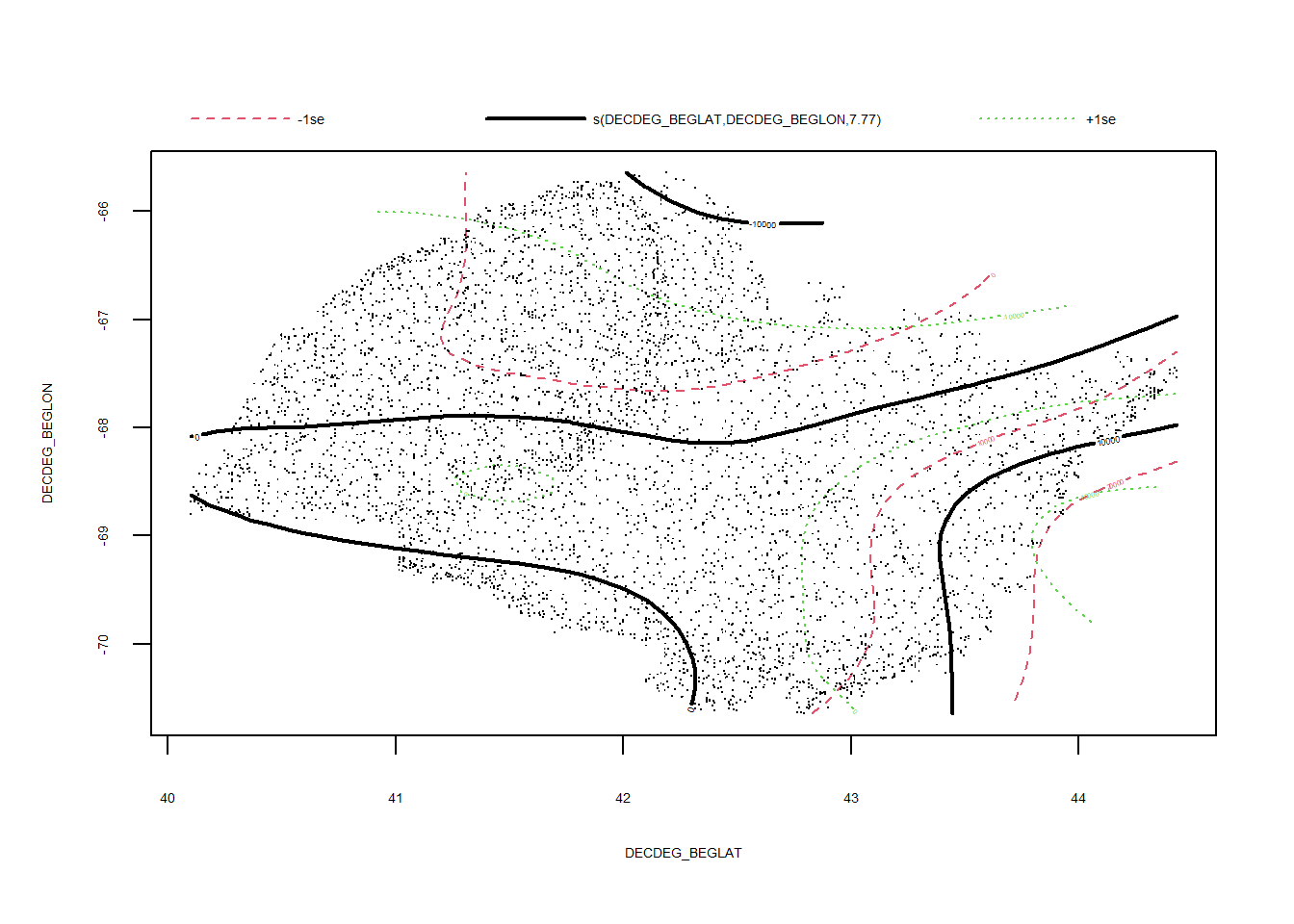
Taxonomic distinctness
FV_GOM_delta_star_SP <- gamm4(delta_star ~ s(FV_bot_temp) + s(FV_surf_temp) + s(FV_bot_sal) +  s(FV_surf_sal) +   s(SETDEPTH)+ s(DECDEG_BEGLAT, DECDEG_BEGLON) , random = ~ (1|EST_YEAR), data = GOM_spring)

gam.check(FV_GOM_delta_star_SP$gam)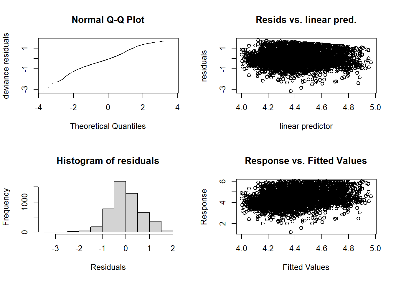
##
## 'gamm' based fit - care required with interpretation.
## Checks based on working residuals may be misleading.
## Basis dimension (k) checking results. Low p-value (k-index<1) may
## indicate that k is too low, especially if edf is close to k'.
##
##                                   k'   edf k-index p-value
## s(FV_bot_temp)                  9.00  1.00    0.97    0.01 **
## s(FV_surf_temp)                 9.00  1.00    0.99    0.26
## s(FV_bot_sal)                   9.00  4.16    0.99    0.32
## s(FV_surf_sal)                  9.00  3.73    1.01    0.67
## s(SETDEPTH)                     9.00  5.23    0.99    0.28
## s(DECDEG_BEGLAT,DECDEG_BEGLON) 29.00 23.21    0.93  <2e-16 ***
## ---
## Signif. codes: 0 '***' 0.001 '**' 0.01 '*' 0.05 '.' 0.1 ' ' 1summary(FV_GOM_delta_star_SP$gam)##
## Family: gaussian
## Link function: identity
##
## Formula:
## delta_star ~ s(FV_bot_temp) + s(FV_surf_temp) + s(FV_bot_sal) +
## s(FV_surf_sal) + s(SETDEPTH) + s(DECDEG_BEGLAT, DECDEG_BEGLON)
##
## Parametric coefficients:
## Estimate Std. Error t value Pr(>|t|)
## (Intercept) 4.3914 0.0299 146.9 <2e-16 ***
## ---
## Signif. codes: 0 '***' 0.001 '**' 0.01 '*' 0.05 '.' 0.1 ' ' 1
##
## Approximate significance of smooth terms:
## edf Ref.df F p-value
## s(FV_bot_temp) 1.000 1.000 16.599 4.69e-05 ***
## s(FV_surf_temp) 1.000 1.000 2.253 0.1334
## s(FV_bot_sal) 4.159 4.159 1.395 0.1658
## s(FV_surf_sal) 3.727 3.727 2.516 0.0588 .
## s(SETDEPTH) 5.232 5.232 6.713 1.82e-06 ***
## s(DECDEG_BEGLAT,DECDEG_BEGLON) 23.214 23.214 7.529 < 2e-16 ***
## ---
## Signif. codes: 0 '***' 0.001 '**' 0.01 '*' 0.05 '.' 0.1 ' ' 1
##
## R-sq.(adj) = 0.0724
## lmer.REML = 9792.6 Scale est. = 0.39141 n = 5038plot(FV_GOM_delta_star_SP$gam)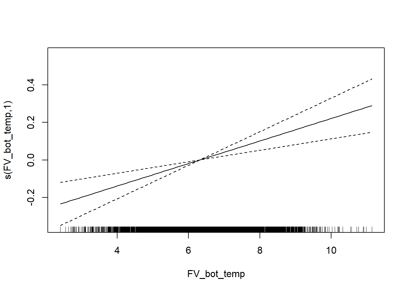
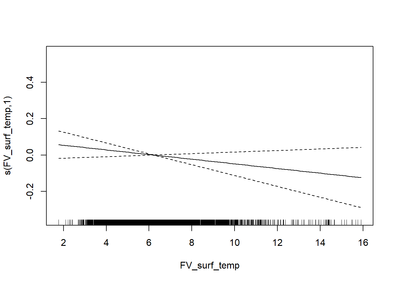
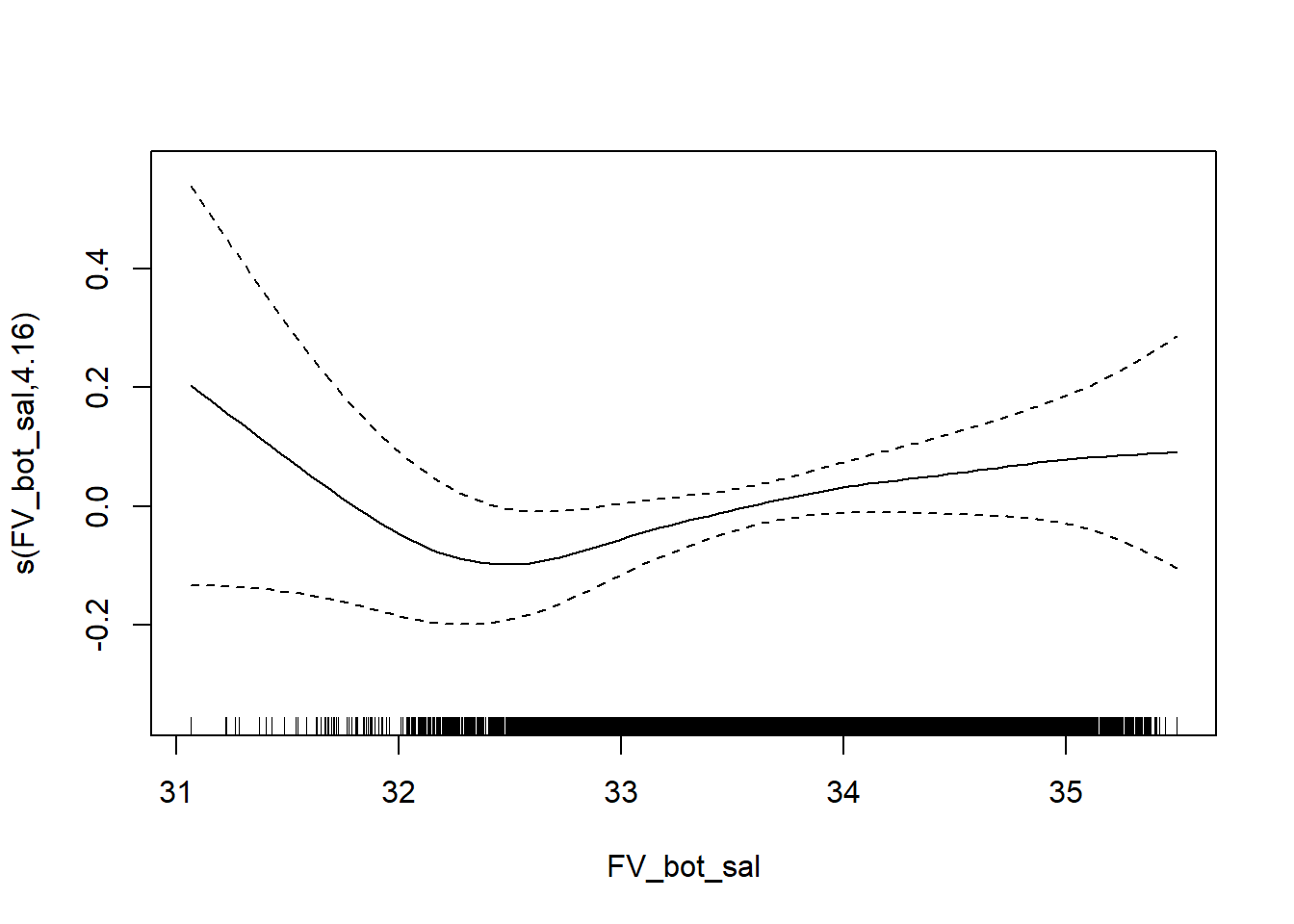
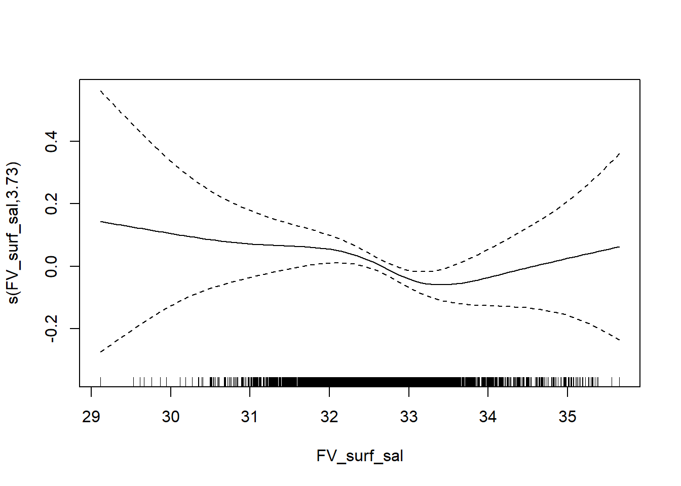
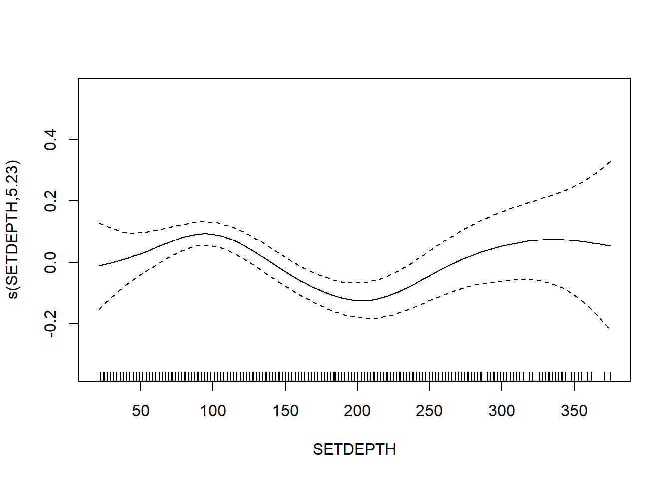
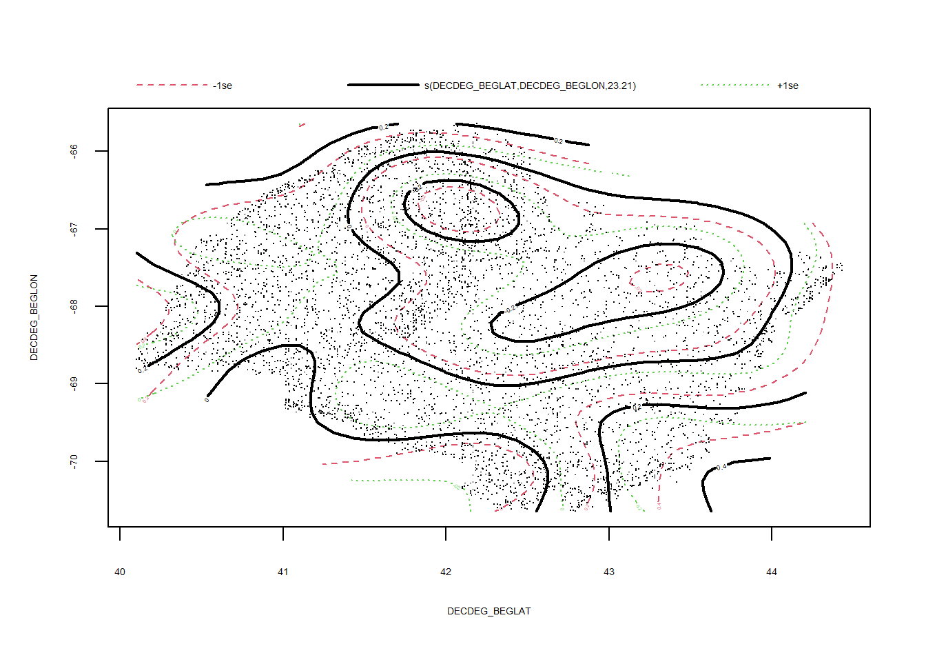
Average taxonomic distinctness
FV_GOM_delta_plus_SP <- gamm4(delta_plus ~ s(FV_bot_temp) + s(FV_surf_temp) + s(FV_bot_sal) +  s(FV_surf_sal) +  s(SETDEPTH)+ s(DECDEG_BEGLAT, DECDEG_BEGLON) , random = ~ (1|EST_YEAR), data = GOM_spring)

gam.check(FV_GOM_delta_plus_SP$gam)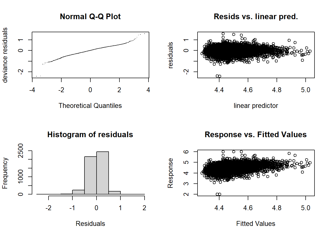
##
## 'gamm' based fit - care required with interpretation.
## Checks based on working residuals may be misleading.
## Basis dimension (k) checking results. Low p-value (k-index<1) may
## indicate that k is too low, especially if edf is close to k'.
##
##                                   k'   edf k-index p-value
## s(FV_bot_temp)                  9.00  5.97    0.98   0.070 .
## s(FV_surf_temp)                 9.00  4.07    0.98   0.060 .
## s(FV_bot_sal)                   9.00  3.15    1.02   0.910
## s(FV_surf_sal)                  9.00  5.67    0.99   0.250
## s(SETDEPTH)                     9.00  5.55    0.98   0.155
## s(DECDEG_BEGLAT,DECDEG_BEGLON) 29.00 24.04    0.98   0.055 .
## ---
## Signif. codes: 0 '***' 0.001 '**' 0.01 '*' 0.05 '.' 0.1 ' ' 1summary(FV_GOM_delta_plus_SP$gam)##
## Family: gaussian
## Link function: identity
##
## Formula:
## delta_plus ~ s(FV_bot_temp) + s(FV_surf_temp) + s(FV_bot_sal) +
## s(FV_surf_sal) + s(SETDEPTH) + s(DECDEG_BEGLAT, DECDEG_BEGLON)
##
## Parametric coefficients:
## Estimate Std. Error t value Pr(>|t|)
## (Intercept) 4.50354 0.02068 217.8 <2e-16 ***
## ---
## Signif. codes: 0 '***' 0.001 '**' 0.01 '*' 0.05 '.' 0.1 ' ' 1
##
## Approximate significance of smooth terms:
## edf Ref.df F p-value
## s(FV_bot_temp) 5.974 5.974 9.238 <2e-16 ***
## s(FV_surf_temp) 4.073 4.073 1.371 0.2154
## s(FV_bot_sal) 3.146 3.146 2.097 0.0726 .
## s(FV_surf_sal) 5.673 5.673 8.251 <2e-16 ***
## s(SETDEPTH) 5.545 5.545 13.201 <2e-16 ***
## s(DECDEG_BEGLAT,DECDEG_BEGLON) 24.044 24.044 8.182 <2e-16 ***
## ---
## Signif. codes: 0 '***' 0.001 '**' 0.01 '*' 0.05 '.' 0.1 ' ' 1
##
## R-sq.(adj) = 0.137
## lmer.REML = 2090.5 Scale est. = 0.083654 n = 5038plot(FV_GOM_delta_plus_SP$gam)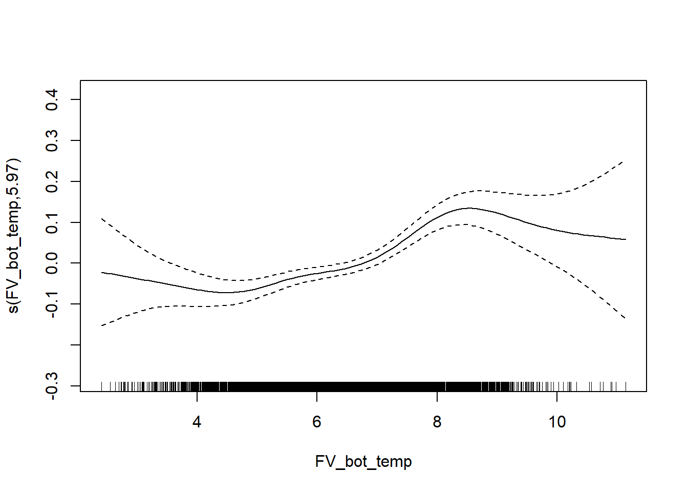
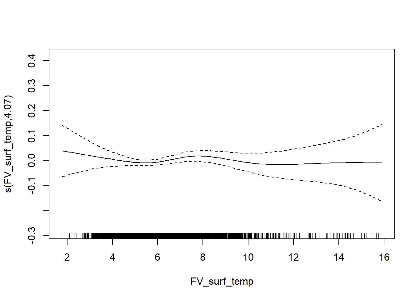
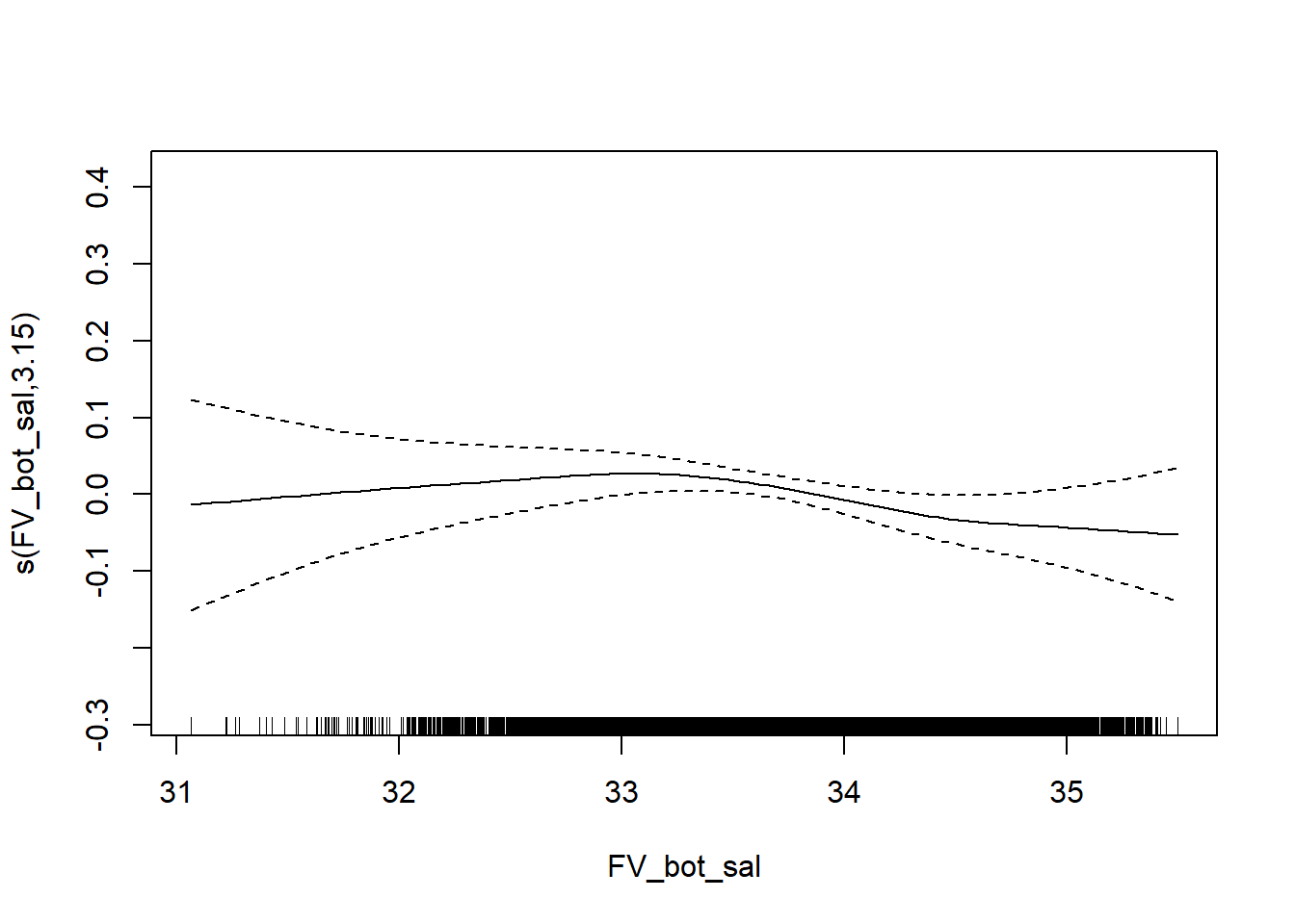
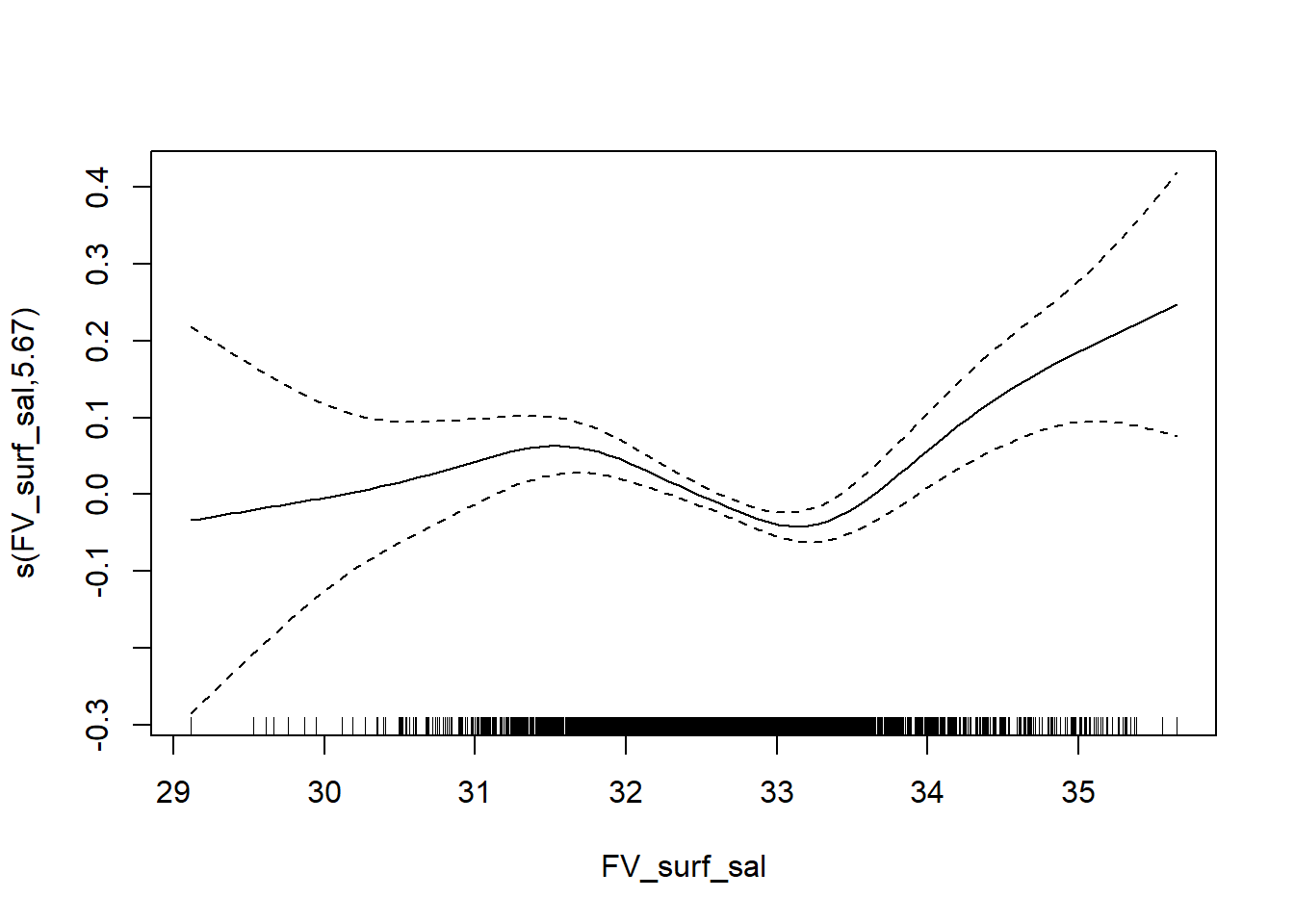
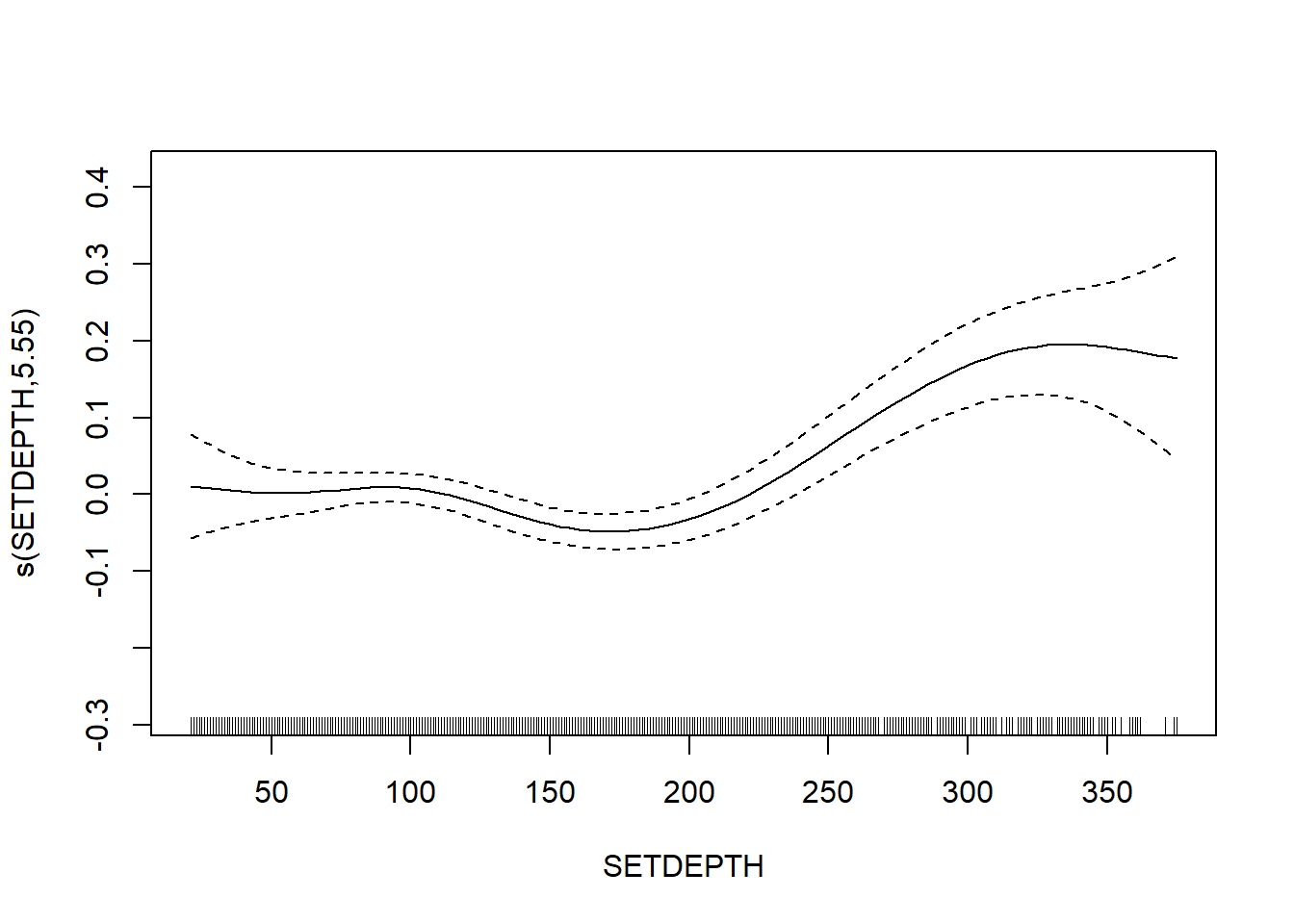
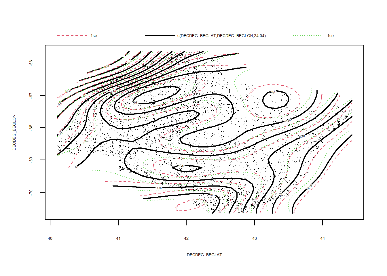
Variation in taxonomic distinctness
FV_GOM_delta_var_SP <- gamm4(delta_var ~ s(FV_bot_temp) + s(FV_surf_temp) + s(FV_bot_sal) +  s(FV_surf_sal) +  s(SETDEPTH)+ s(DECDEG_BEGLAT, DECDEG_BEGLON) , random = ~ (1|EST_YEAR), data = GOM_spring)

gam.check(FV_GOM_delta_var_SP$gam)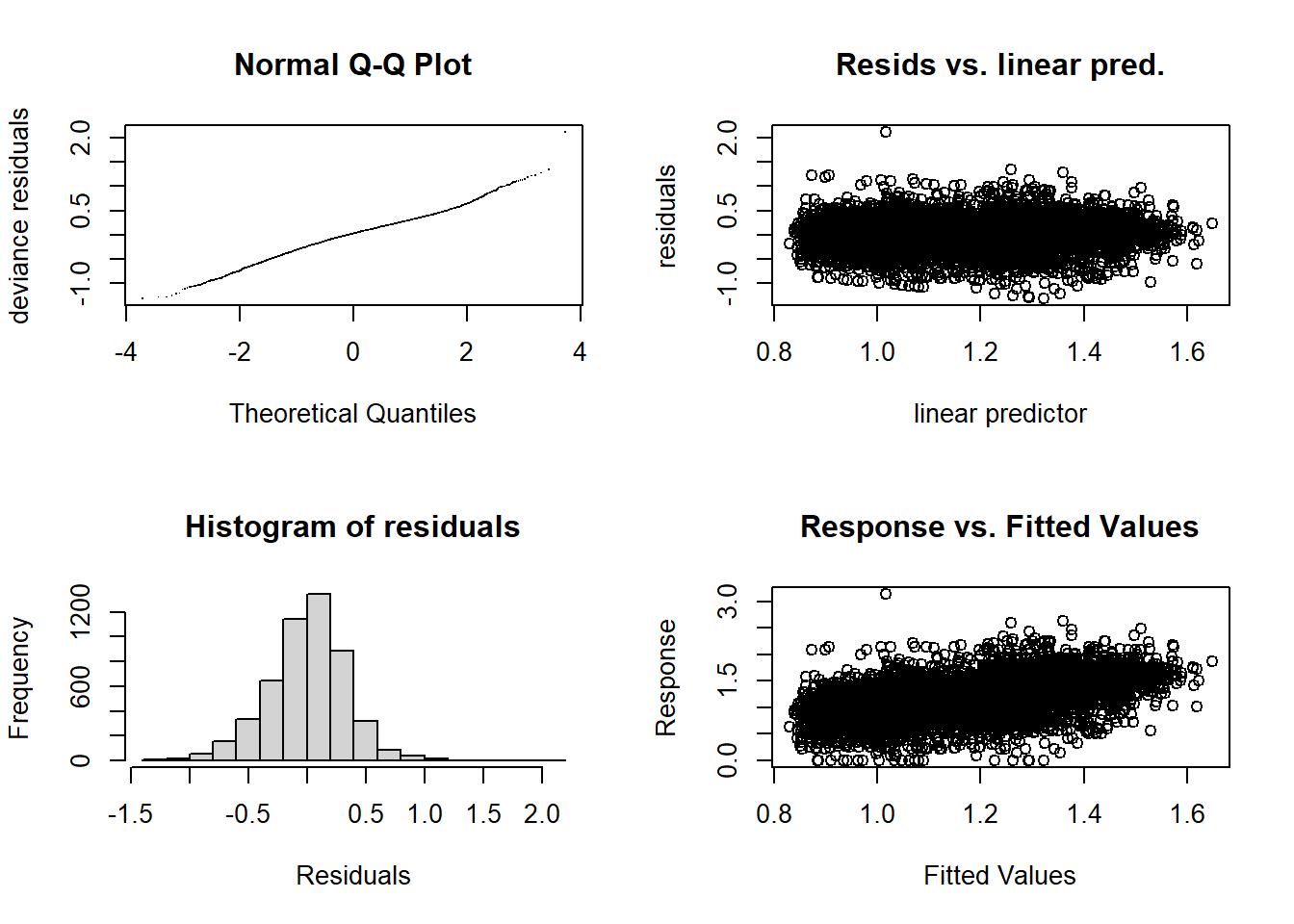
##
## 'gamm' based fit - care required with interpretation.
## Checks based on working residuals may be misleading.
## Basis dimension (k) checking results. Low p-value (k-index<1) may
## indicate that k is too low, especially if edf is close to k'.
##
##                                   k'   edf k-index p-value
## s(FV_bot_temp)                  9.00  1.00    0.97    0.03 *
## s(FV_surf_temp)                 9.00  1.00    1.01    0.70
## s(FV_bot_sal)                   9.00  2.11    1.00    0.54
## s(FV_surf_sal)                  9.00  4.68    0.99    0.23
## s(SETDEPTH)                     9.00  4.94    0.99    0.18
## s(DECDEG_BEGLAT,DECDEG_BEGLON) 29.00 24.58    0.98    0.02 *
## ---
## Signif. codes: 0 '***' 0.001 '**' 0.01 '*' 0.05 '.' 0.1 ' ' 1summary(FV_GOM_delta_var_SP$gam)##
## Family: gaussian
## Link function: identity
##
## Formula:
## delta_var ~ s(FV_bot_temp) + s(FV_surf_temp) + s(FV_bot_sal) +
## s(FV_surf_sal) + s(SETDEPTH) + s(DECDEG_BEGLAT, DECDEG_BEGLON)
##
## Parametric coefficients:
## Estimate Std. Error t value Pr(>|t|)
## (Intercept) 1.17996 0.01764 66.91 <2e-16 ***
## ---
## Signif. codes: 0 '***' 0.001 '**' 0.01 '*' 0.05 '.' 0.1 ' ' 1
##
## Approximate significance of smooth terms:
## edf Ref.df F p-value
## s(FV_bot_temp) 1.000 1.000 9.644 0.001910 **
## s(FV_surf_temp) 1.000 1.000 9.416 0.002162 **
## s(FV_bot_sal) 2.111 2.111 0.806 0.395671
## s(FV_surf_sal) 4.684 4.684 4.535 0.000844 ***
## s(SETDEPTH) 4.943 4.943 20.858 < 2e-16 ***
## s(DECDEG_BEGLAT,DECDEG_BEGLON) 24.584 24.584 15.432 < 2e-16 ***
## ---
## Signif. codes: 0 '***' 0.001 '**' 0.01 '*' 0.05 '.' 0.1 ' ' 1
##
## R-sq.(adj) = 0.21
## lmer.REML = 3003.5 Scale est. = 0.10117 n = 5038plot(FV_GOM_delta_var_SP$gam)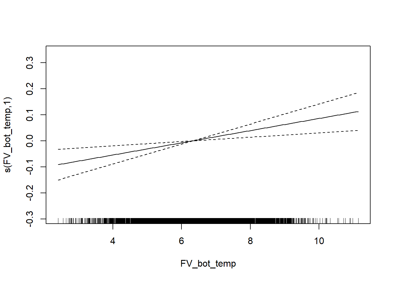
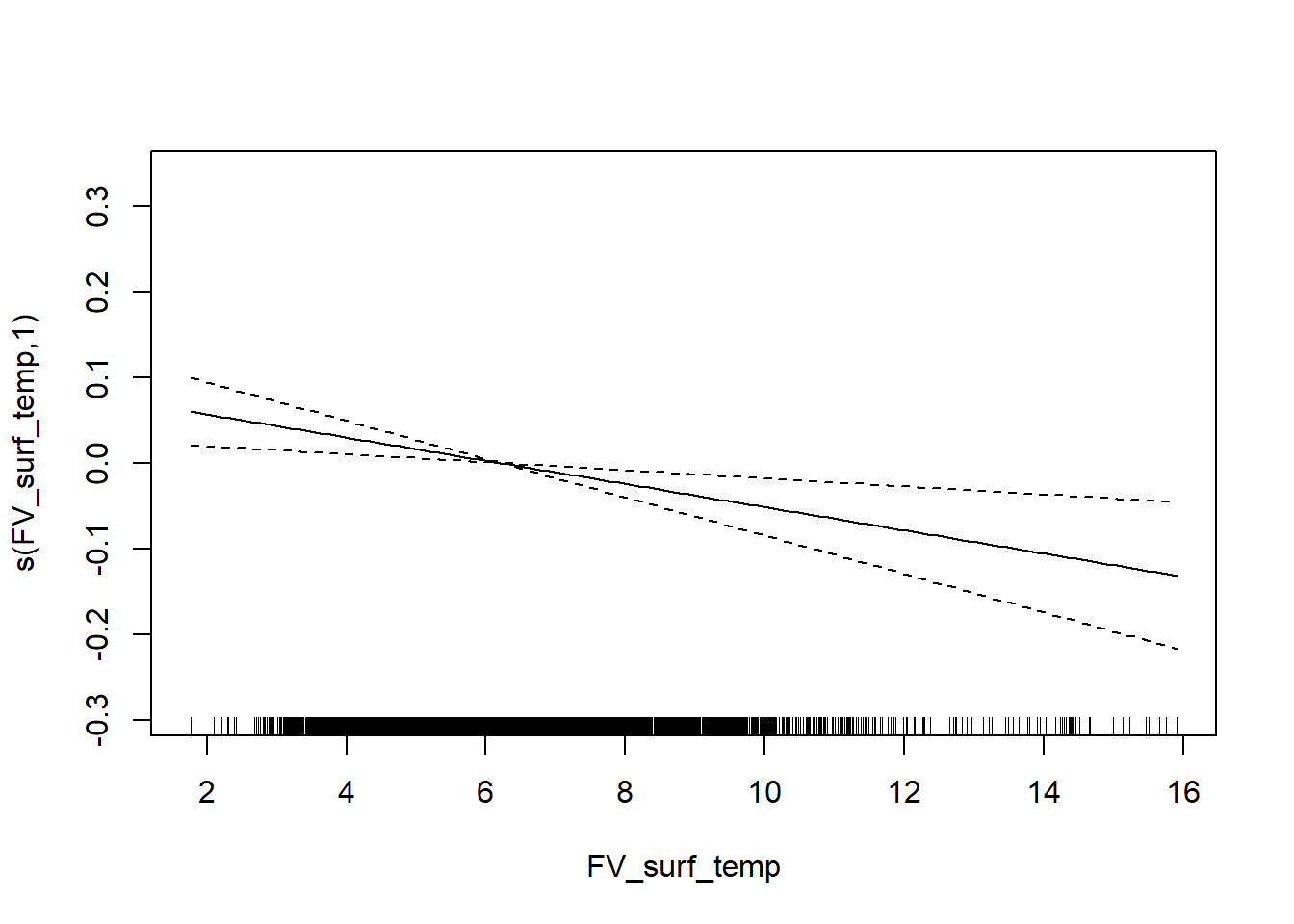
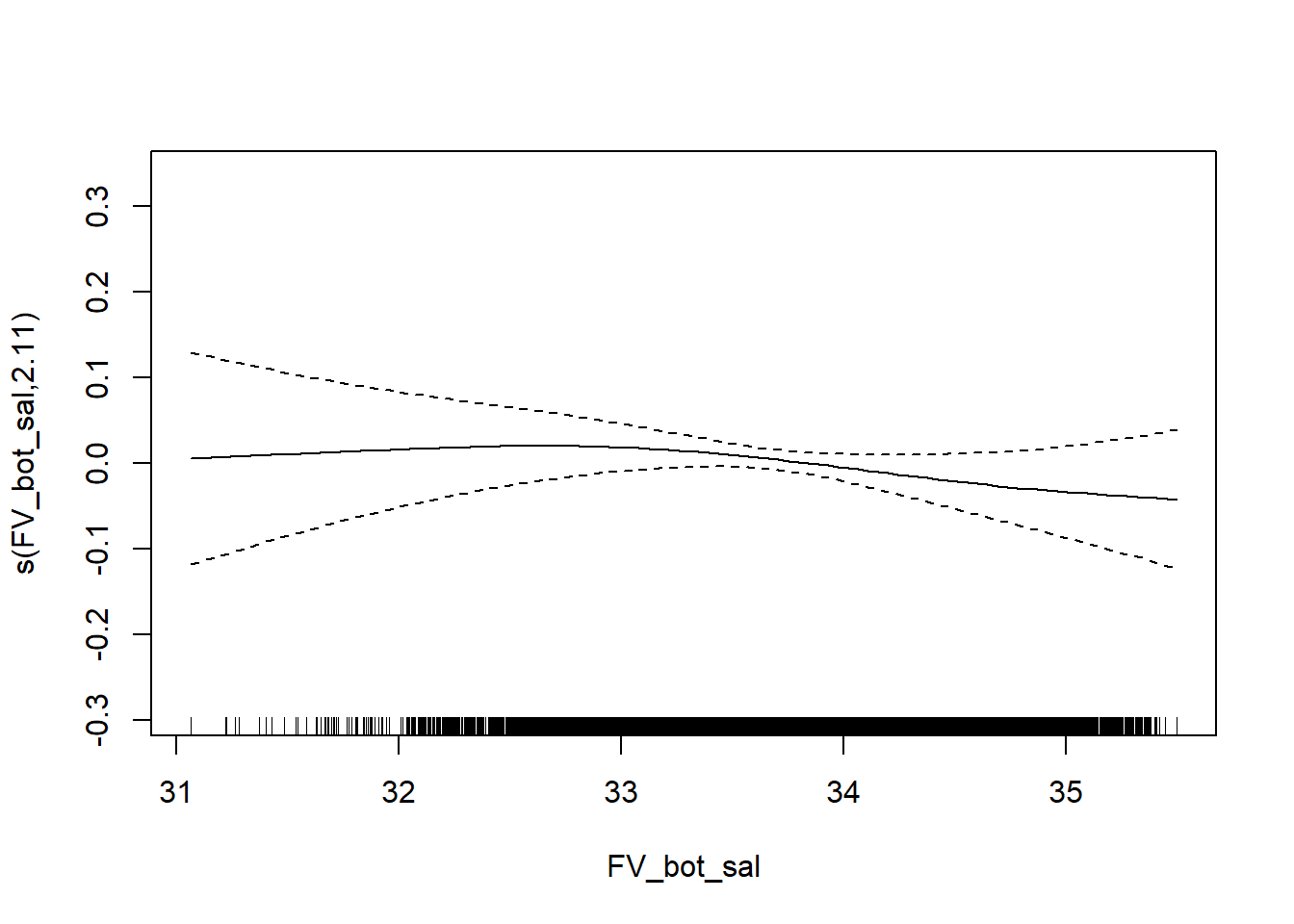
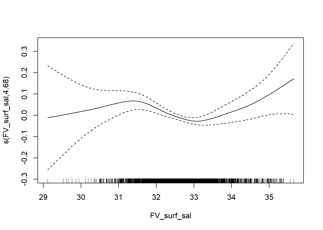
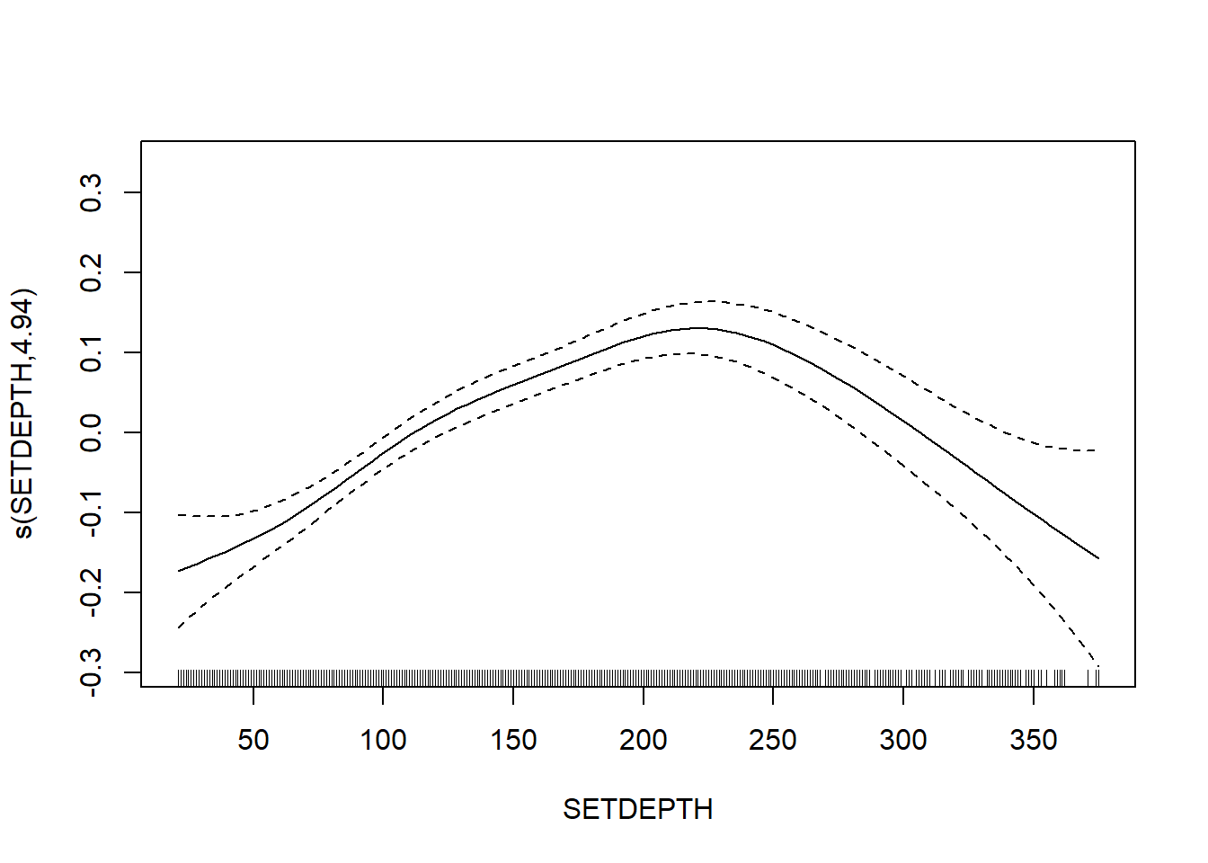
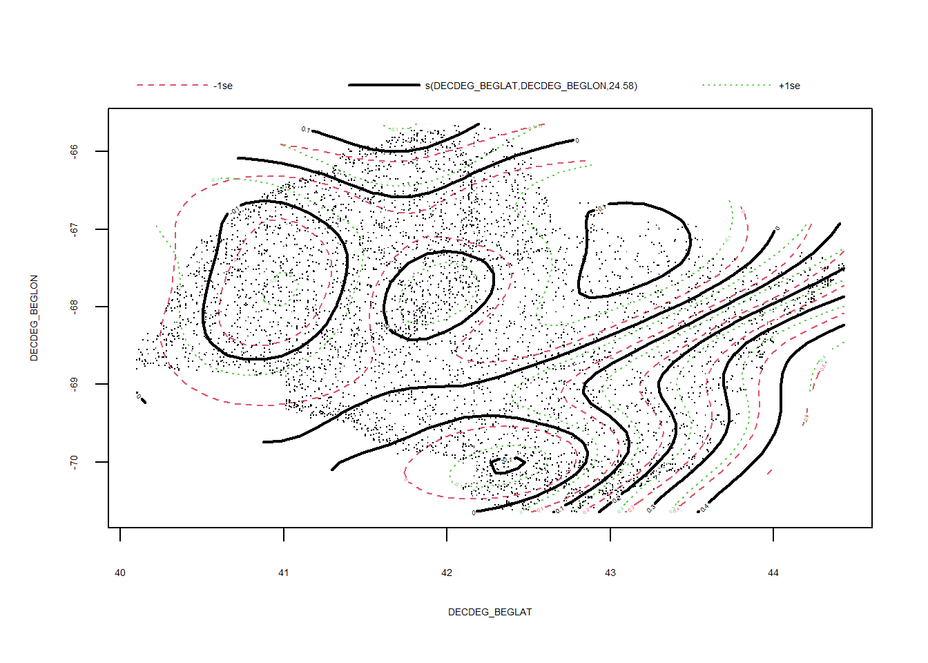
Fall MADMF GAMMs
- all with FVCOM data
setwd("C:/Users/jjesse/Box/Kerr Lab/Fisheries Science Lab/ME NH Trawl- Seagrant/Seagrant-AEW/Results/GAMMs")

MA_fall <- read.csv("MA_fall_full.csv")

MA_spring <- read.csv("MA_spring_full.csv")
Species richness
library(gamm4)
# number of species
FV_MA_N_FL <- gamm4(N_species ~ s(FV_bot_temp) + s(FV_surf_temp) + s(FV_bot_sal) +  s(FV_surf_sal) + s(DEPTH_M)+ s(LATITUDE, LONGITUDE) , random = ~ (1|YEAR), data = MA_fall)

gam.check(FV_MA_N_FL$gam)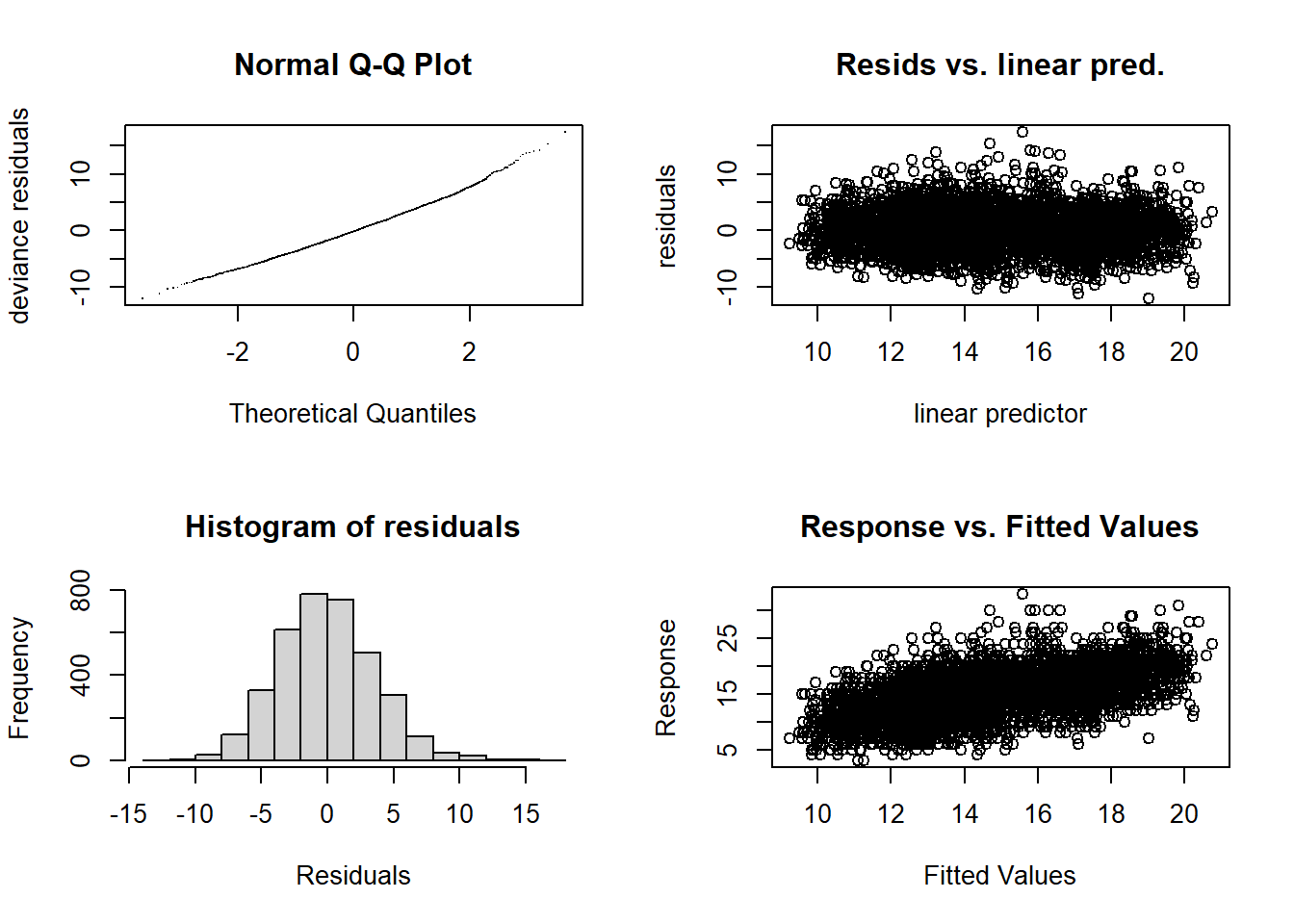
##
## 'gamm' based fit - care required with interpretation.
## Checks based on working residuals may be misleading.
## Basis dimension (k) checking results. Low p-value (k-index<1) may
## indicate that k is too low, especially if edf is close to k'.
##
##                          k'   edf k-index p-value
## s(FV_bot_temp)         9.00  4.59    1.01    0.79
## s(FV_surf_temp)        9.00  3.07    1.00    0.40
## s(FV_bot_sal)          9.00  2.12    0.99    0.34
## s(FV_surf_sal)         9.00  4.42    0.99    0.23
## s(DEPTH_M)             9.00  6.00    0.90  <2e-16 ***
## s(LATITUDE,LONGITUDE) 29.00 26.59    0.88  <2e-16 ***
## ---
## Signif. codes: 0 '***' 0.001 '**' 0.01 '*' 0.05 '.' 0.1 ' ' 1summary(FV_MA_N_FL$gam)##
## Family: gaussian
## Link function: identity
##
## Formula:
## N_species ~ s(FV_bot_temp) + s(FV_surf_temp) + s(FV_bot_sal) +
## s(FV_surf_sal) + s(DEPTH_M) + s(LATITUDE, LONGITUDE)
##
## Parametric coefficients:
## Estimate Std. Error t value Pr(>|t|)
## (Intercept) 14.6227 0.1937 75.47 <2e-16 ***
## ---
## Signif. codes: 0 '***' 0.001 '**' 0.01 '*' 0.05 '.' 0.1 ' ' 1
##
## Approximate significance of smooth terms:
## edf Ref.df F p-value
## s(FV_bot_temp) 4.590 4.590 4.636 0.00667 **
## s(FV_surf_temp) 3.072 3.072 1.989 0.08939 .
## s(FV_bot_sal) 2.119 2.119 0.293 0.66174
## s(FV_surf_sal) 4.415 4.415 2.020 0.06811 .
## s(DEPTH_M) 6.000 6.000 22.340 < 2e-16 ***
## s(LATITUDE,LONGITUDE) 26.591 26.591 16.652 < 2e-16 ***
## ---
## Signif. codes: 0 '***' 0.001 '**' 0.01 '*' 0.05 '.' 0.1 ' ' 1
##
## R-sq.(adj) = 0.317
## lmer.REML = 19657 Scale est. = 12.272 n = 3635plot(FV_MA_N_FL$gam)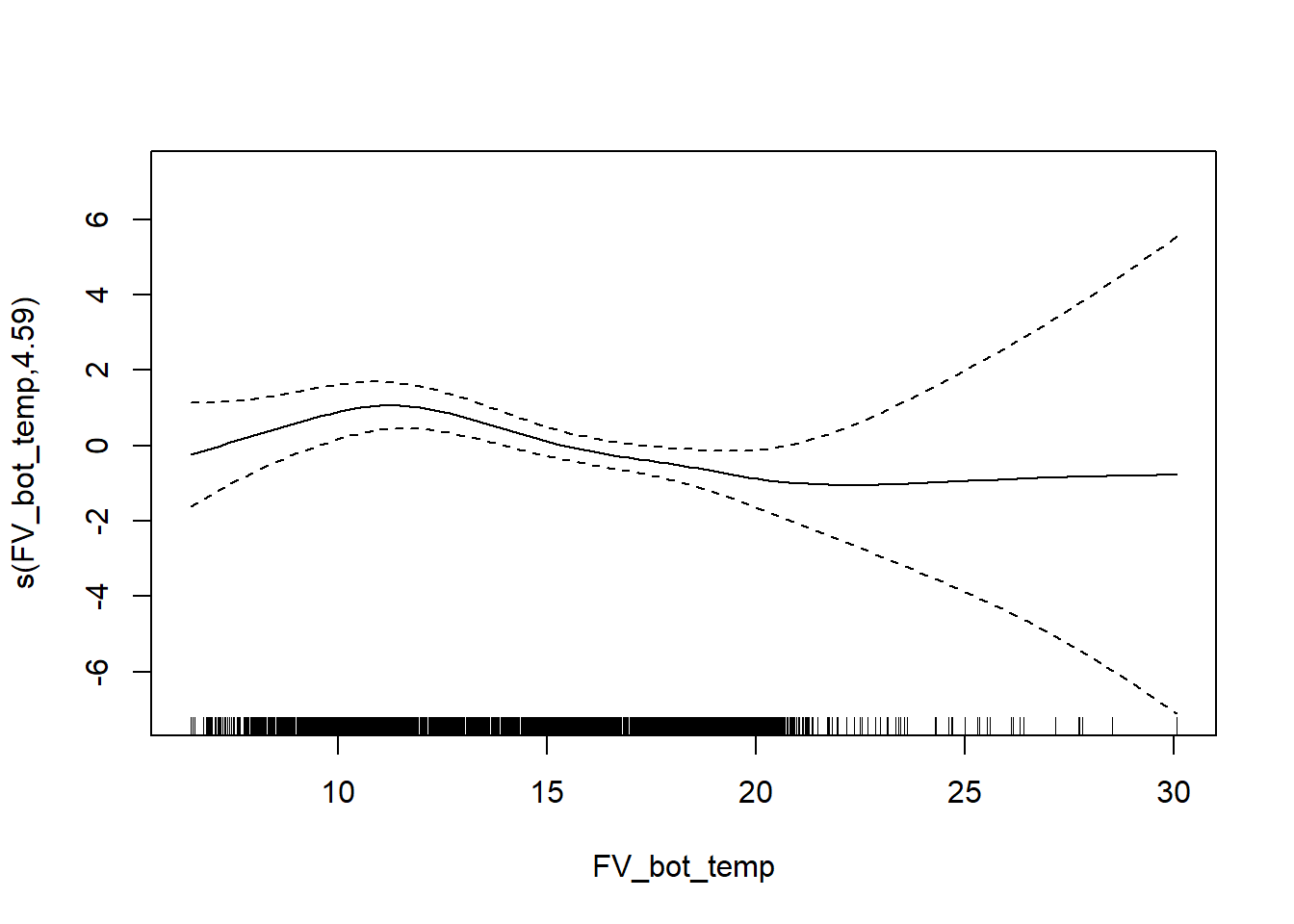
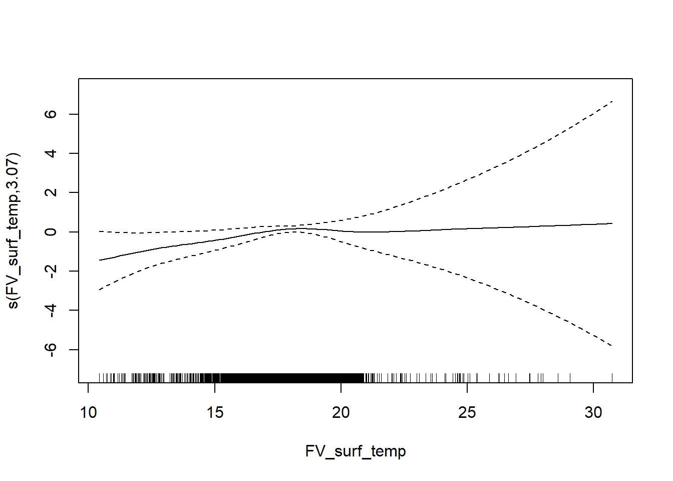
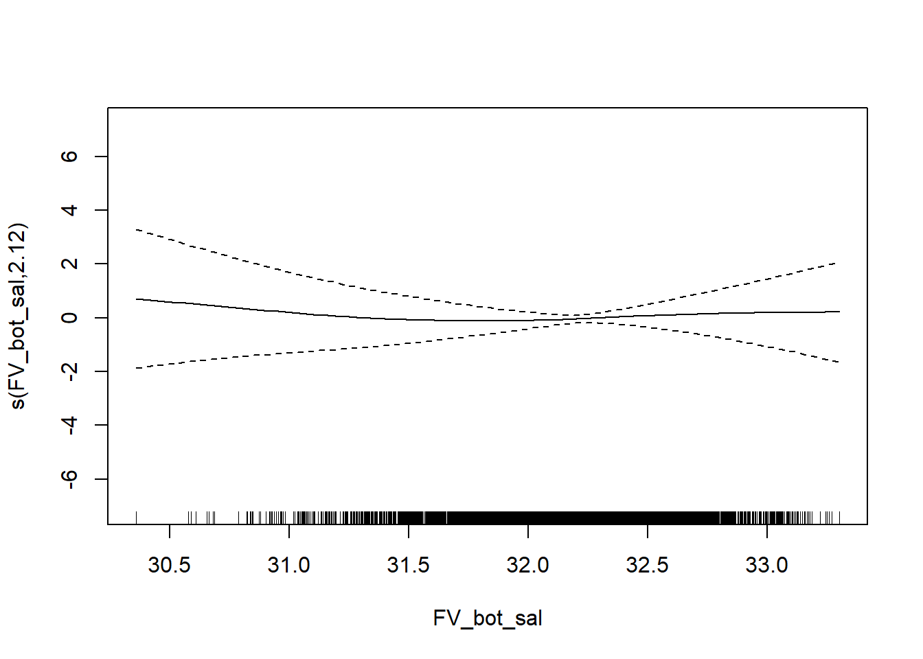
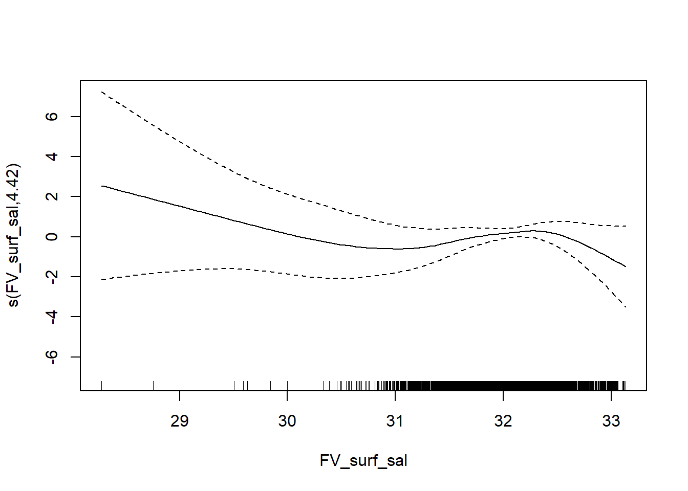
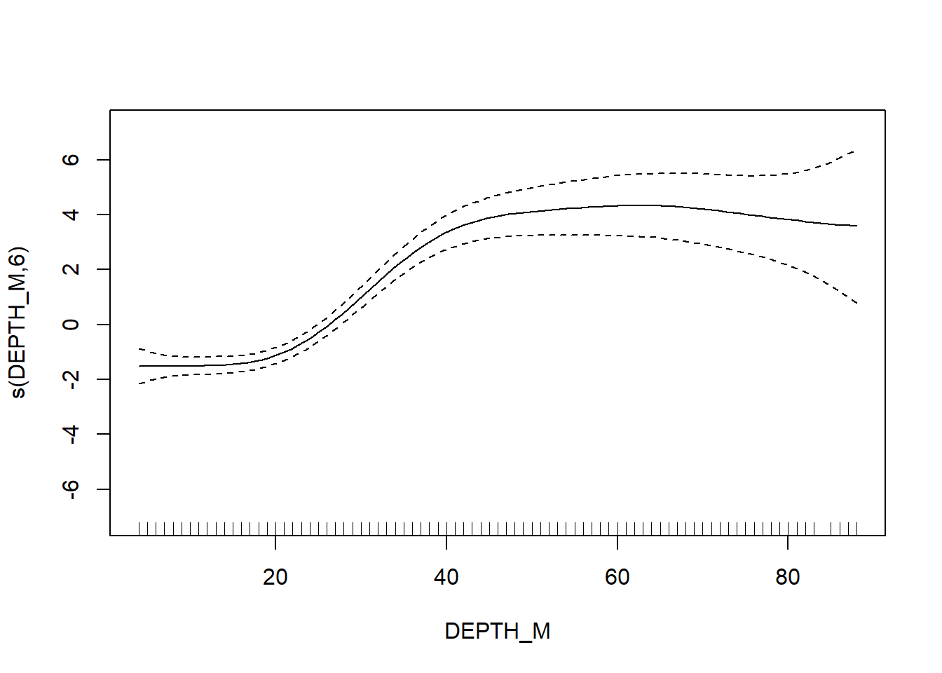
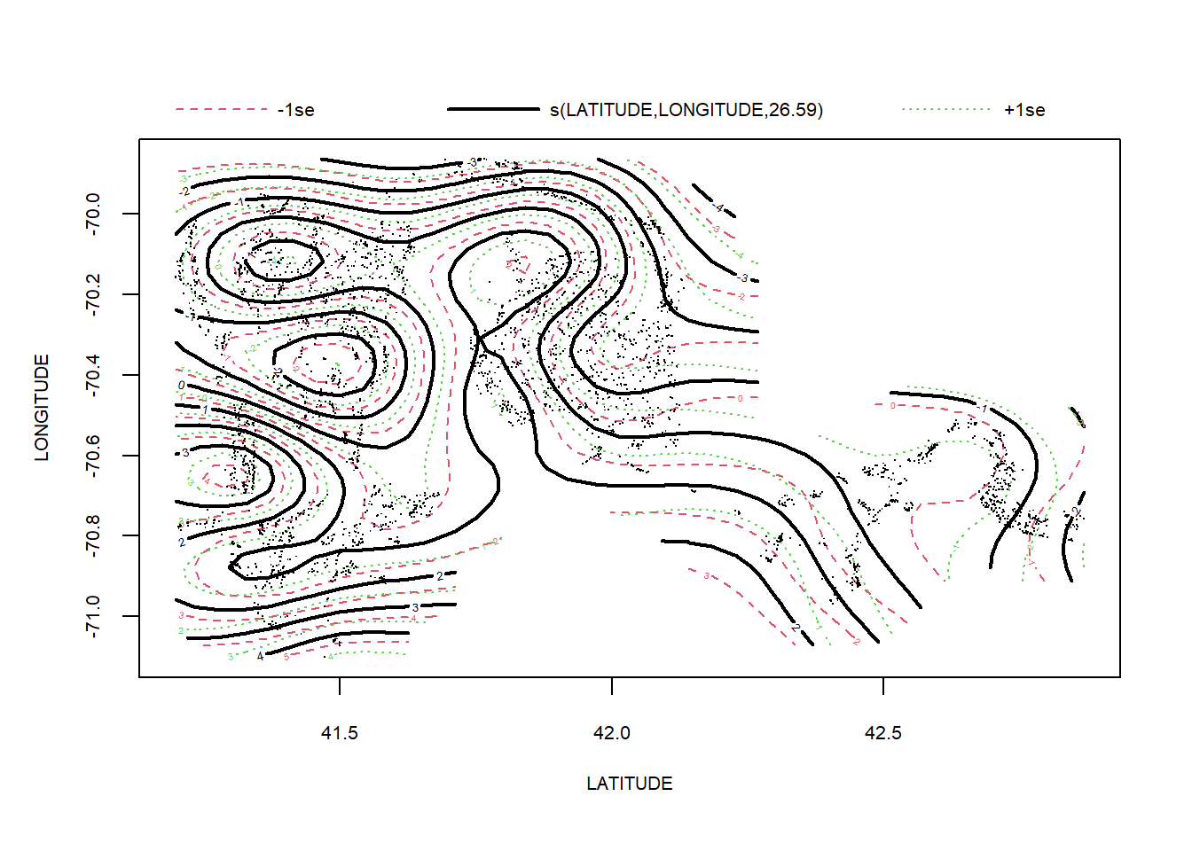
Shannon-Weiner diversity
# S-W
FV_MA_H_FL <- gamm4(H_index ~ s(FV_bot_temp) + s(FV_surf_temp) + s(FV_bot_sal) +  s(FV_surf_sal) +  s(DEPTH_M)+ s(LATITUDE, LONGITUDE) , random = ~ (1|YEAR), data = MA_fall)

gam.check(FV_MA_H_FL$gam)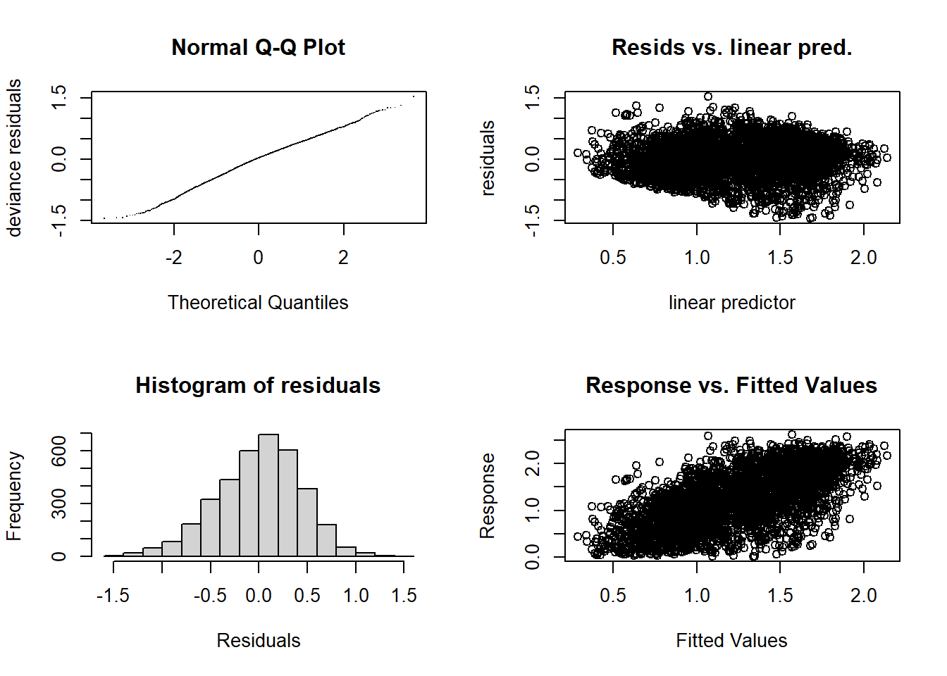
##
## 'gamm' based fit - care required with interpretation.
## Checks based on working residuals may be misleading.
## Basis dimension (k) checking results. Low p-value (k-index<1) may
## indicate that k is too low, especially if edf is close to k'.
##
##                          k'   edf k-index p-value
## s(FV_bot_temp)         9.00  3.78    0.99   0.215
## s(FV_surf_temp)        9.00  4.48    1.00   0.485
## s(FV_bot_sal)          9.00  2.38    0.99   0.375
## s(FV_surf_sal)         9.00  1.00    0.98   0.095 .
## s(DEPTH_M)             9.00  5.77    0.94  <2e-16 ***
## s(LATITUDE,LONGITUDE) 29.00 26.30    0.90  <2e-16 ***
## ---
## Signif. codes: 0 '***' 0.001 '**' 0.01 '*' 0.05 '.' 0.1 ' ' 1summary(FV_MA_H_FL$gam)##
## Family: gaussian
## Link function: identity
##
## Formula:
## H_index ~ s(FV_bot_temp) + s(FV_surf_temp) + s(FV_bot_sal) +
## s(FV_surf_sal) + s(DEPTH_M) + s(LATITUDE, LONGITUDE)
##
## Parametric coefficients:
## Estimate Std. Error t value Pr(>|t|)
## (Intercept) 1.25872 0.01521 82.78 <2e-16 ***
## ---
## Signif. codes: 0 '***' 0.001 '**' 0.01 '*' 0.05 '.' 0.1 ' ' 1
##
## Approximate significance of smooth terms:
## edf Ref.df F p-value
## s(FV_bot_temp) 3.776 3.776 6.395 0.000139 ***
## s(FV_surf_temp) 4.483 4.483 1.708 0.194021
## s(FV_bot_sal) 2.378 2.378 2.317 0.157322
## s(FV_surf_sal) 1.000 1.000 0.053 0.817116
## s(DEPTH_M) 5.771 5.771 17.225 < 2e-16 ***
## s(LATITUDE,LONGITUDE) 26.302 26.302 12.817 < 2e-16 ***
## ---
## Signif. codes: 0 '***' 0.001 '**' 0.01 '*' 0.05 '.' 0.1 ' ' 1
##
## R-sq.(adj) = 0.419
## lmer.REML = 4449.8 Scale est. = 0.18764 n = 3635plot(FV_MA_H_FL$gam)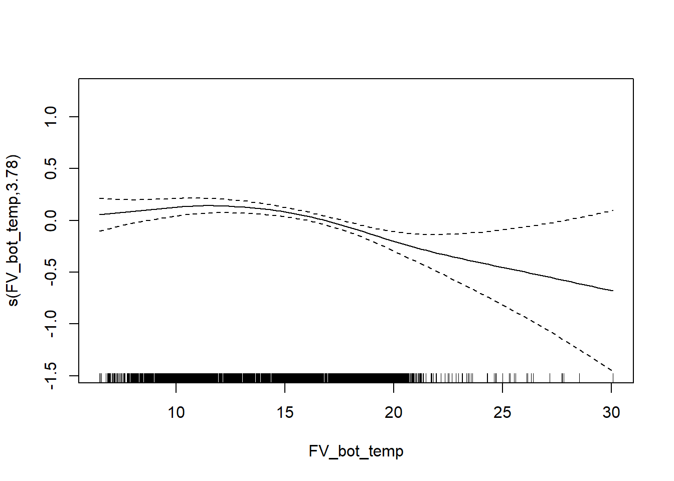
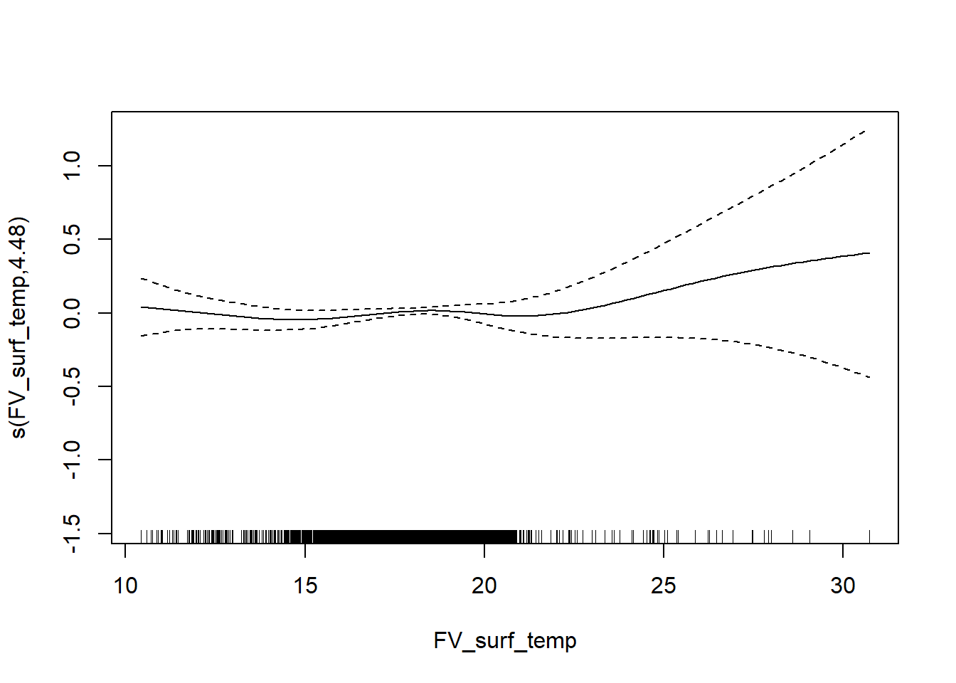
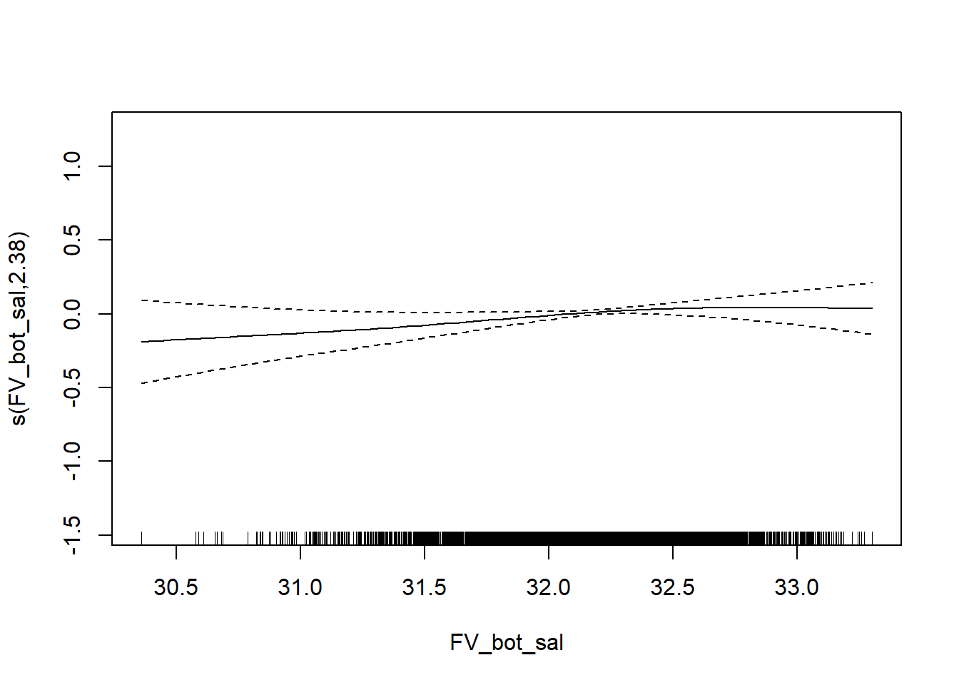
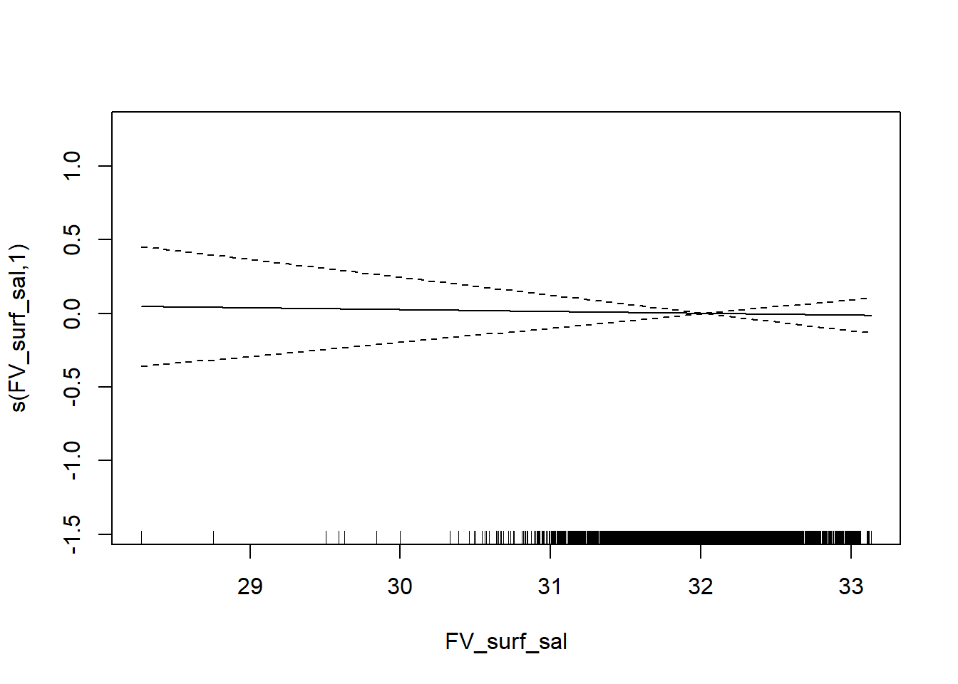
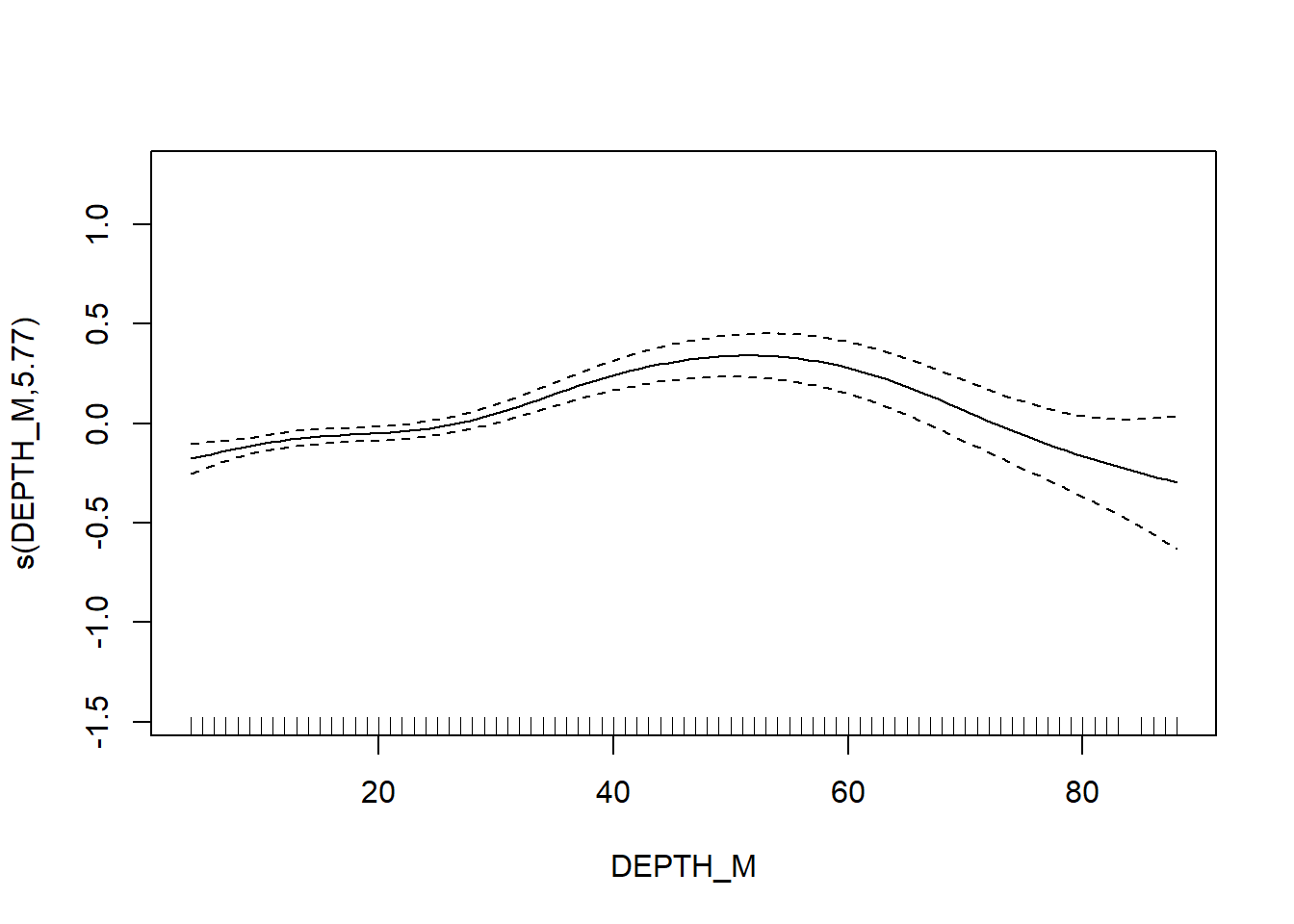
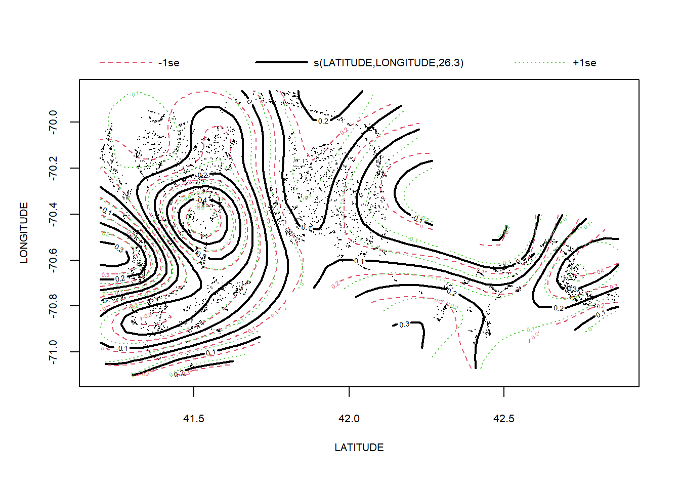
Simpson’s diveristy
# Simpsons D
FV_MA_D_FL <- gamm4(D_index ~ s(FV_bot_temp) + s(FV_surf_temp) + s(FV_bot_sal) +  s(FV_surf_sal) +  s(DEPTH_M)+ s(LATITUDE, LONGITUDE) , random = ~ (1|YEAR), data = MA_fall)

gam.check(FV_MA_D_FL$gam)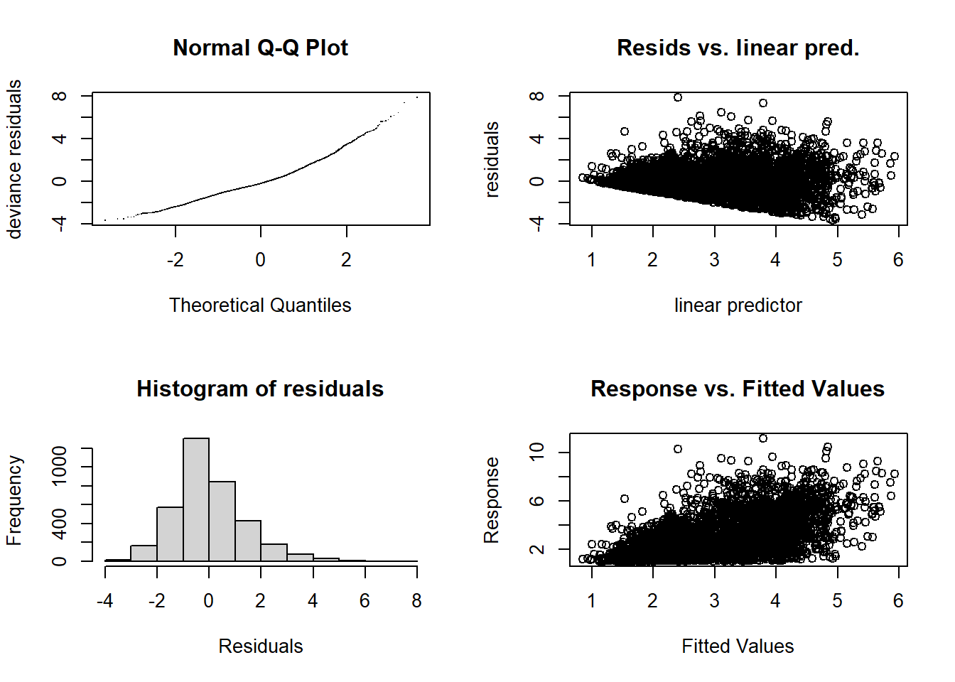
##
## 'gamm' based fit - care required with interpretation.
## Checks based on working residuals may be misleading.
## Basis dimension (k) checking results. Low p-value (k-index<1) may
## indicate that k is too low, especially if edf is close to k'.
##
##                          k'   edf k-index p-value
## s(FV_bot_temp)         9.00  4.17    0.99    0.26
## s(FV_surf_temp)        9.00  4.02    0.98    0.12
## s(FV_bot_sal)          9.00  1.19    0.99    0.23
## s(FV_surf_sal)         9.00  1.00    0.99    0.35
## s(DEPTH_M)             9.00  6.32    0.94  <2e-16 ***
## s(LATITUDE,LONGITUDE) 29.00 25.36    0.94  <2e-16 ***
## ---
## Signif. codes: 0 '***' 0.001 '**' 0.01 '*' 0.05 '.' 0.1 ' ' 1summary(FV_MA_D_FL$gam)##
## Family: gaussian
## Link function: identity
##
## Formula:
## D_index ~ s(FV_bot_temp) + s(FV_surf_temp) + s(FV_bot_sal) +
## s(FV_surf_sal) + s(DEPTH_M) + s(LATITUDE, LONGITUDE)
##
## Parametric coefficients:
## Estimate Std. Error t value Pr(>|t|)
## (Intercept) 2.99939 0.04777 62.79 <2e-16 ***
## ---
## Signif. codes: 0 '***' 0.001 '**' 0.01 '*' 0.05 '.' 0.1 ' ' 1
##
## Approximate significance of smooth terms:
## edf Ref.df F p-value
## s(FV_bot_temp) 4.172 4.172 6.368 9e-05 ***
## s(FV_surf_temp) 4.017 4.017 2.002 0.101
## s(FV_bot_sal) 1.192 1.192 0.317 0.719
## s(FV_surf_sal) 1.000 1.000 0.623 0.430
## s(DEPTH_M) 6.324 6.324 23.306 <2e-16 ***
## s(LATITUDE,LONGITUDE) 25.361 25.361 8.783 <2e-16 ***
## ---
## Signif. codes: 0 '***' 0.001 '**' 0.01 '*' 0.05 '.' 0.1 ' ' 1
##
## R-sq.(adj) = 0.327
## lmer.REML = 12777 Scale est. = 1.8684 n = 3635plot(FV_MA_D_FL$gam)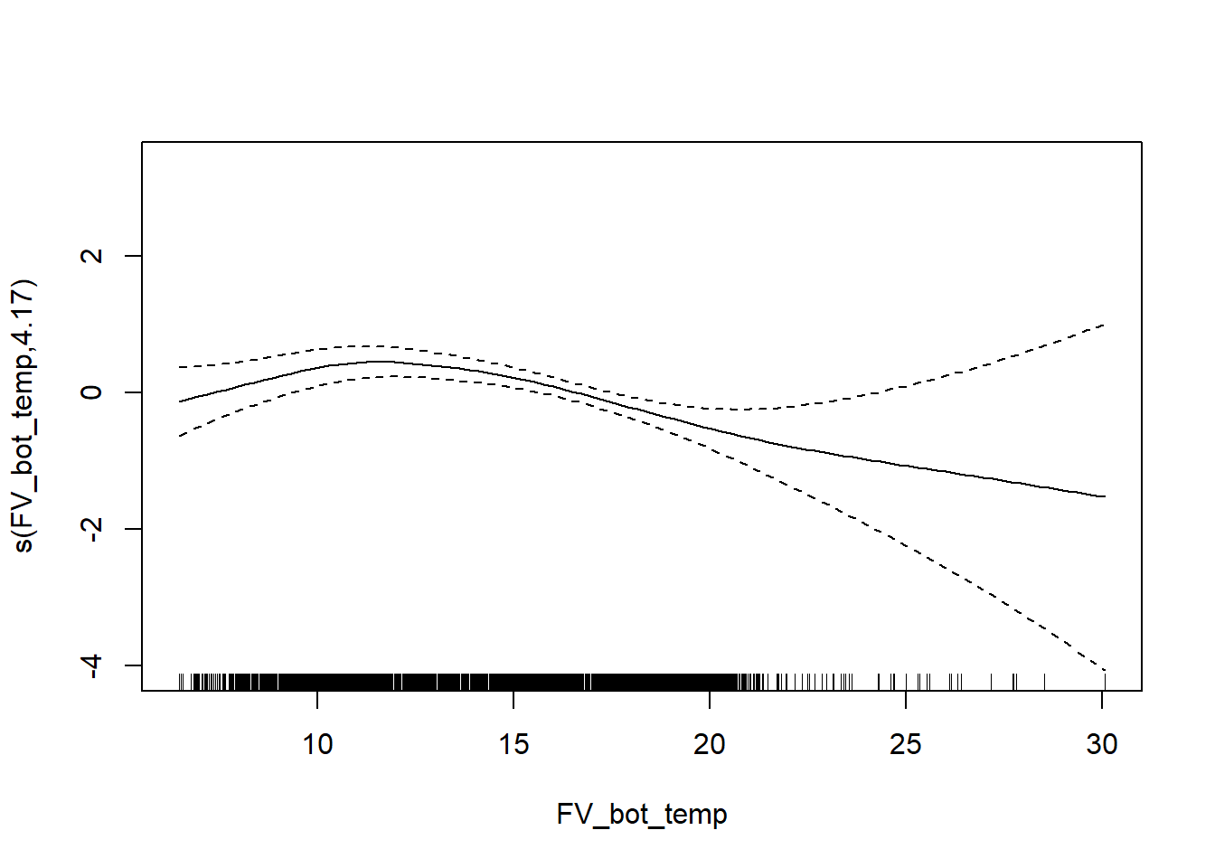

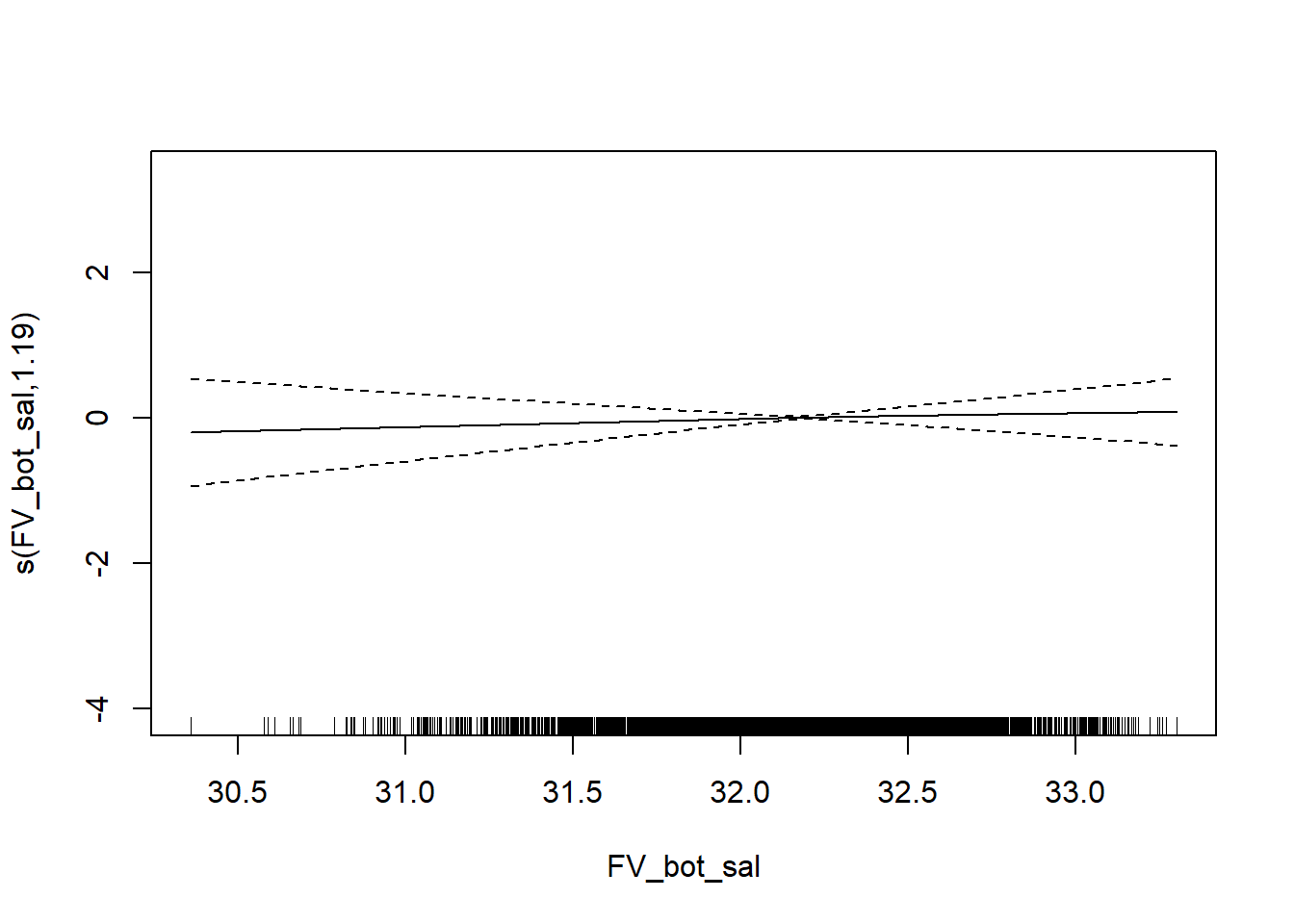
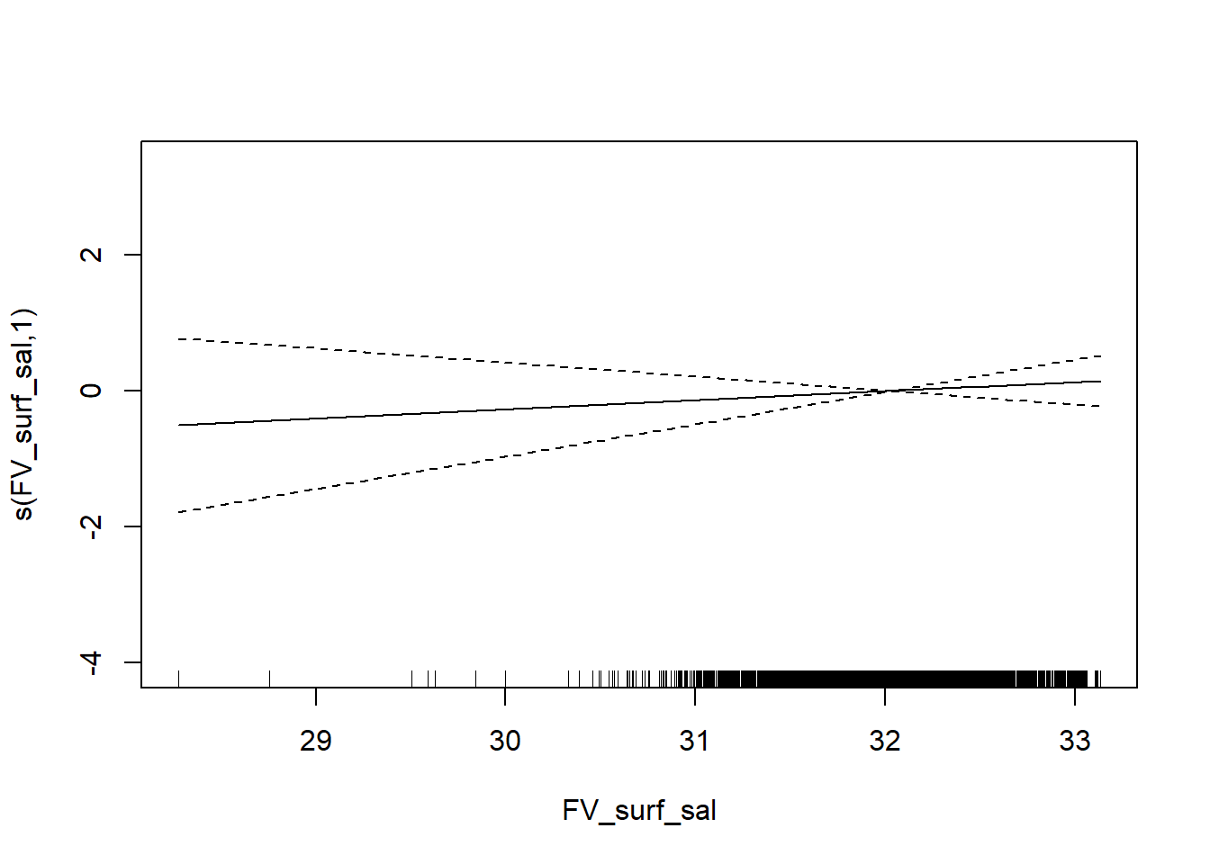
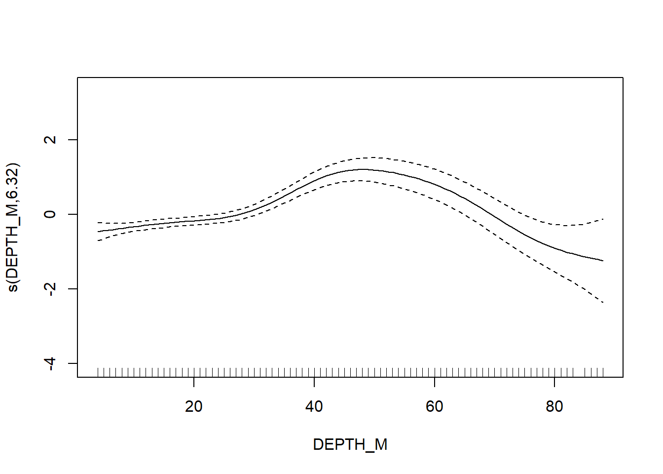
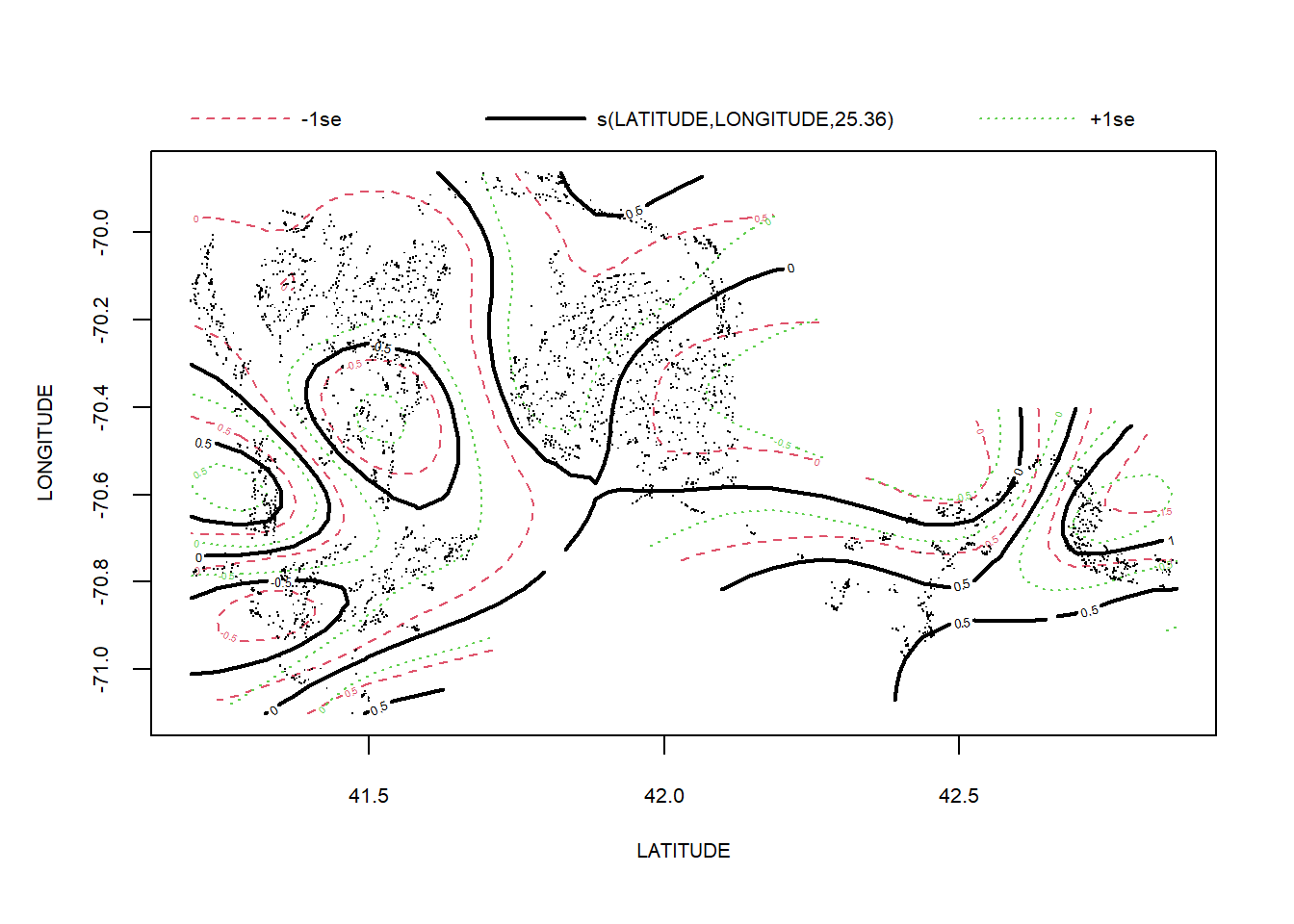
Simpson’s Evenness
#simpsons e
FV_MA_E_FL <- gamm4(E_index ~ s(FV_bot_temp) + s(FV_surf_temp) + s(FV_bot_sal) +  s(FV_surf_sal) + s(DEPTH_M)+ s(LATITUDE, LONGITUDE) , random = ~ (1|YEAR), data = MA_fall)

gam.check(FV_MA_E_FL$gam)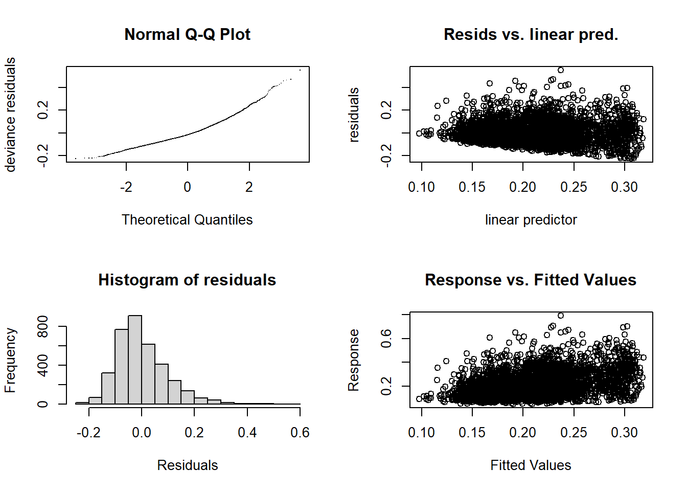
##
## 'gamm' based fit - care required with interpretation.
## Checks based on working residuals may be misleading.
## Basis dimension (k) checking results. Low p-value (k-index<1) may
## indicate that k is too low, especially if edf is close to k'.
##
##                          k'   edf k-index p-value
## s(FV_bot_temp)         9.00  2.99    0.99    0.32
## s(FV_surf_temp)        9.00  1.56    1.01    0.66
## s(FV_bot_sal)          9.00  1.00    0.99    0.35
## s(FV_surf_sal)         9.00  2.06    0.99    0.34
## s(DEPTH_M)             9.00  5.39    0.96    0.01 **
## s(LATITUDE,LONGITUDE) 29.00 21.96    0.95  <2e-16 ***
## ---
## Signif. codes: 0 '***' 0.001 '**' 0.01 '*' 0.05 '.' 0.1 ' ' 1summary(FV_MA_E_FL$gam)##
## Family: gaussian
## Link function: identity
##
## Formula:
## E_index ~ s(FV_bot_temp) + s(FV_surf_temp) + s(FV_bot_sal) +
## s(FV_surf_sal) + s(DEPTH_M) + s(LATITUDE, LONGITUDE)
##
## Parametric coefficients:
## Estimate Std. Error t value Pr(>|t|)
## (Intercept) 0.210254 0.002704 77.76 <2e-16 ***
## ---
## Signif. codes: 0 '***' 0.001 '**' 0.01 '*' 0.05 '.' 0.1 ' ' 1
##
## Approximate significance of smooth terms:
## edf Ref.df F p-value
## s(FV_bot_temp) 2.990 2.990 3.543 0.0156 *
## s(FV_surf_temp) 1.560 1.560 0.253 0.7932
## s(FV_bot_sal) 1.000 1.000 0.017 0.8951
## s(FV_surf_sal) 2.056 2.056 0.843 0.3619
## s(DEPTH_M) 5.387 5.387 10.277 <2e-16 ***
## s(LATITUDE,LONGITUDE) 21.964 21.964 8.653 <2e-16 ***
## ---
## Signif. codes: 0 '***' 0.001 '**' 0.01 '*' 0.05 '.' 0.1 ' ' 1
##
## R-sq.(adj) = 0.177
## lmer.REML = -6541.4 Scale est. = 0.0092084 n = 3635plot(FV_MA_E_FL$gam)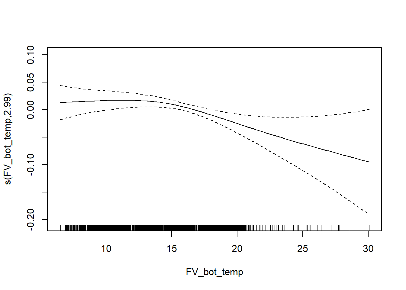
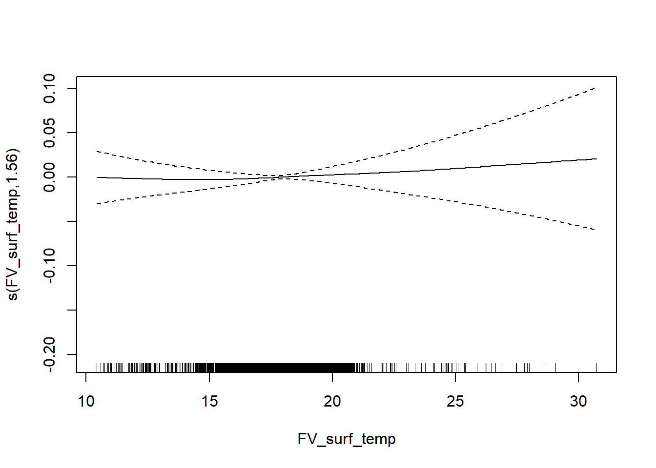
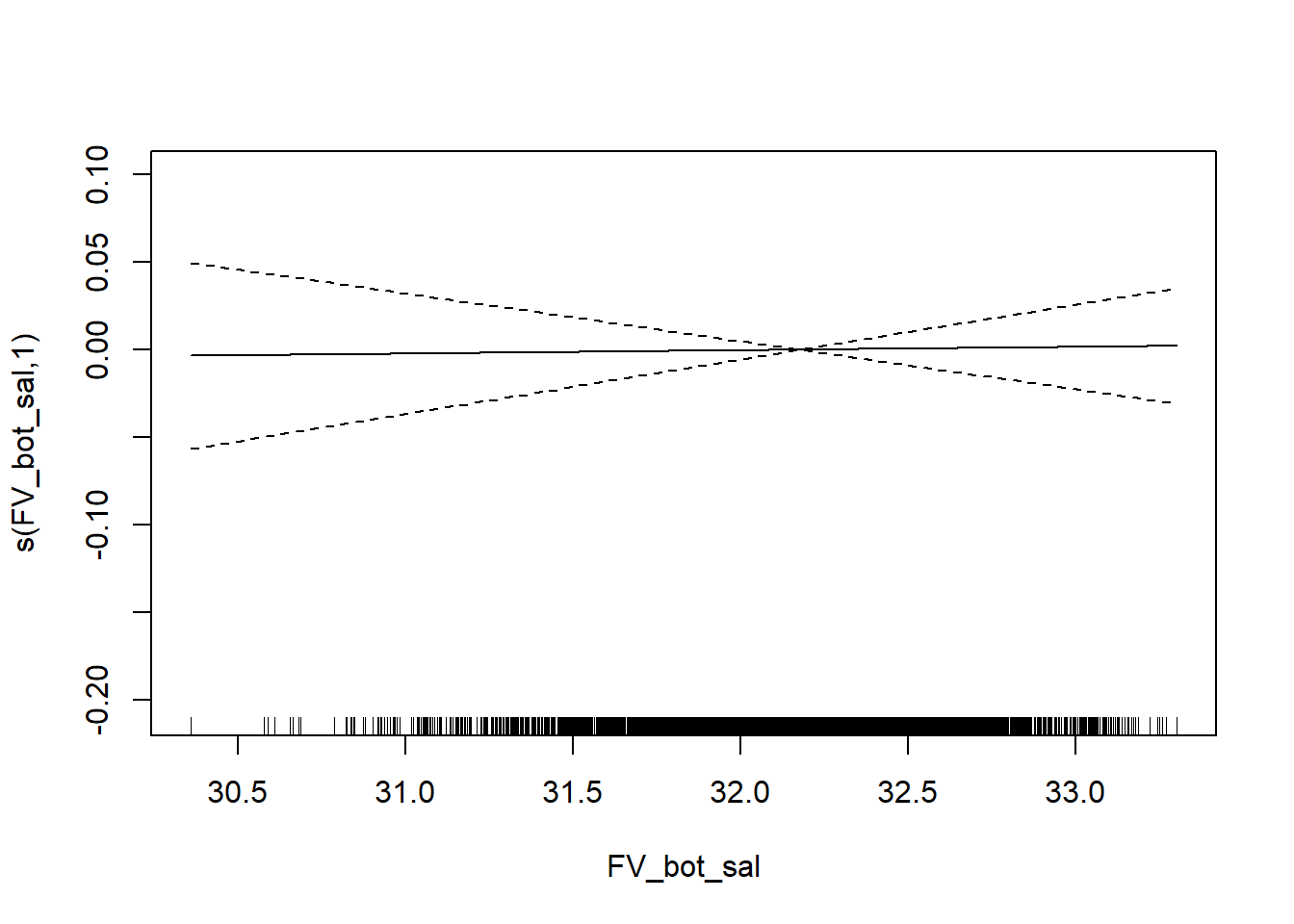
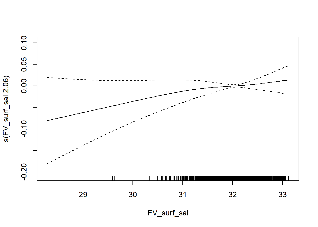
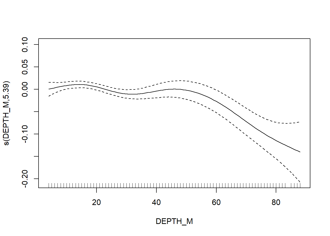
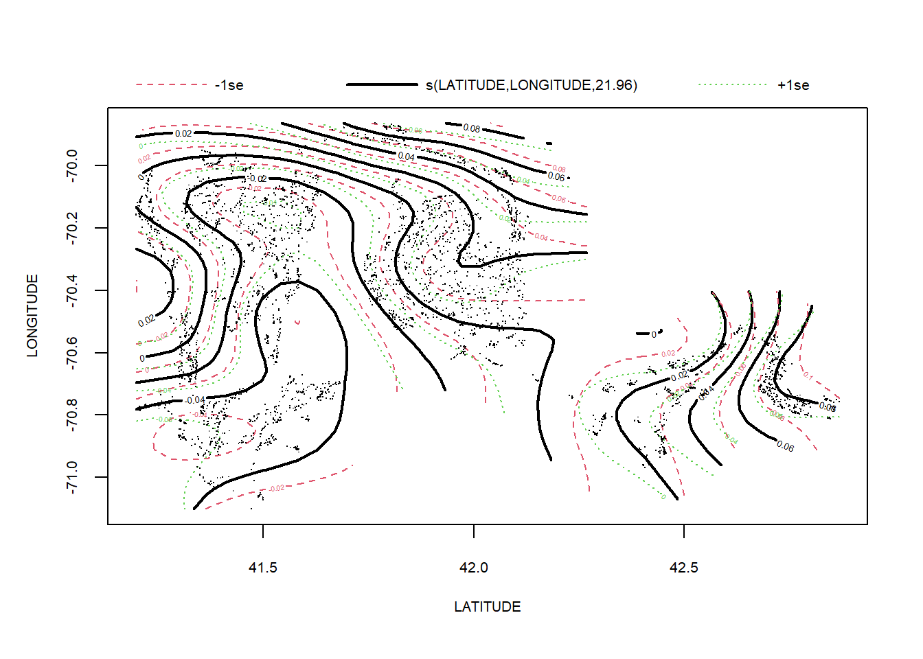
Taxonomic diversity
#tax diversity
FV_MA_delta_FL <- gamm4(delta ~ s(FV_bot_temp) + s(FV_surf_temp) + s(FV_bot_sal) +  s(FV_surf_sal) +  s(DEPTH_M)+ s(LATITUDE, LONGITUDE) , random = ~ (1|YEAR), data = MA_fall)

gam.check(FV_MA_delta_FL$gam)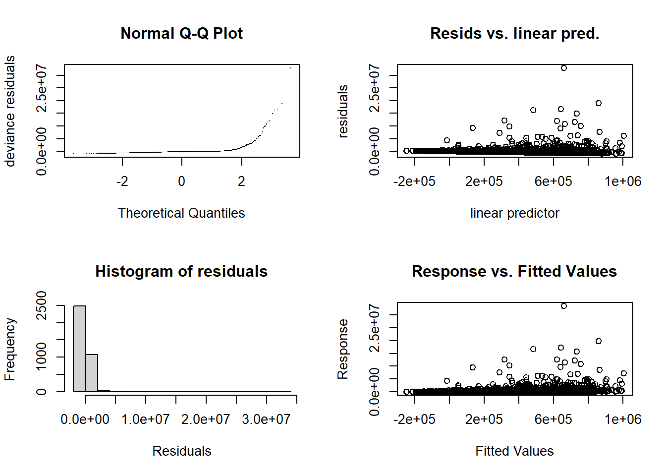
##
## 'gamm' based fit - care required with interpretation.
## Checks based on working residuals may be misleading.
## Basis dimension (k) checking results. Low p-value (k-index<1) may
## indicate that k is too low, especially if edf is close to k'.
##
##                          k'   edf k-index p-value
## s(FV_bot_temp)         9.00  2.85    1.00   0.465
## s(FV_surf_temp)        9.00  1.90    1.01   0.700
## s(FV_bot_sal)          9.00  1.60    0.94   0.005 **
## s(FV_surf_sal)         9.00  1.00    1.01   0.590
## s(DEPTH_M)             9.00  2.48    0.97   0.030 *
## s(LATITUDE,LONGITUDE) 29.00 17.82    1.00   0.570
## ---
## Signif. codes: 0 '***' 0.001 '**' 0.01 '*' 0.05 '.' 0.1 ' ' 1summary(FV_MA_delta_FL$gam)##
## Family: gaussian
## Link function: identity
##
## Formula:
## delta ~ s(FV_bot_temp) + s(FV_surf_temp) + s(FV_bot_sal) + s(FV_surf_sal) +
## s(DEPTH_M) + s(LATITUDE, LONGITUDE)
##
## Parametric coefficients:
## Estimate Std. Error t value Pr(>|t|)
## (Intercept) 239001 29054 8.226 2.67e-16 ***
## ---
## Signif. codes: 0 '***' 0.001 '**' 0.01 '*' 0.05 '.' 0.1 ' ' 1
##
## Approximate significance of smooth terms:
## edf Ref.df F p-value
## s(FV_bot_temp) 2.850 2.850 5.001 0.00262 **
## s(FV_surf_temp) 1.896 1.896 0.205 0.83902
## s(FV_bot_sal) 1.599 1.599 0.807 0.55624
## s(FV_surf_sal) 1.000 1.000 0.106 0.74526
## s(DEPTH_M) 2.477 2.477 4.097 0.02409 *
## s(LATITUDE,LONGITUDE) 17.824 17.824 4.104 < 2e-16 ***
## ---
## Signif. codes: 0 '***' 0.001 '**' 0.01 '*' 0.05 '.' 0.1 ' ' 1
##
## R-sq.(adj) = 0.0588
## lmer.REML = 1.1107e+05 Scale est. = 1.1711e+12 n = 3630plot(FV_MA_delta_FL$gam)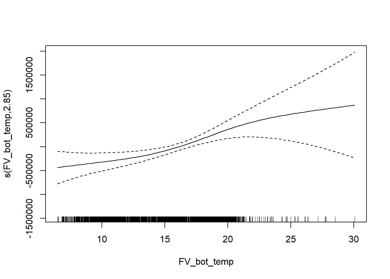
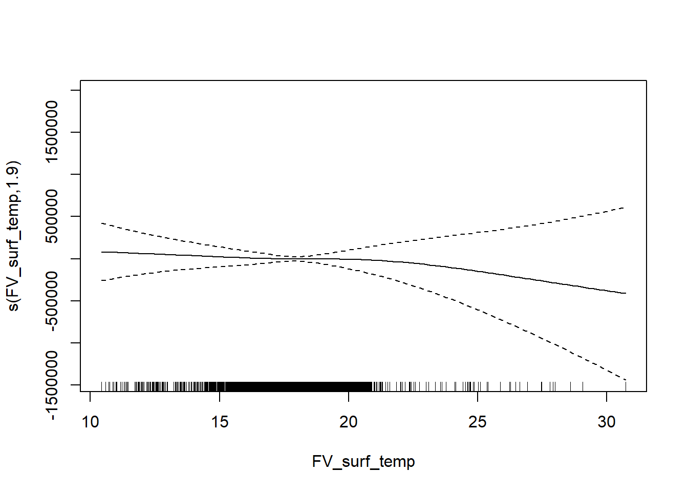
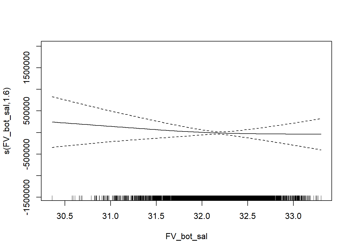
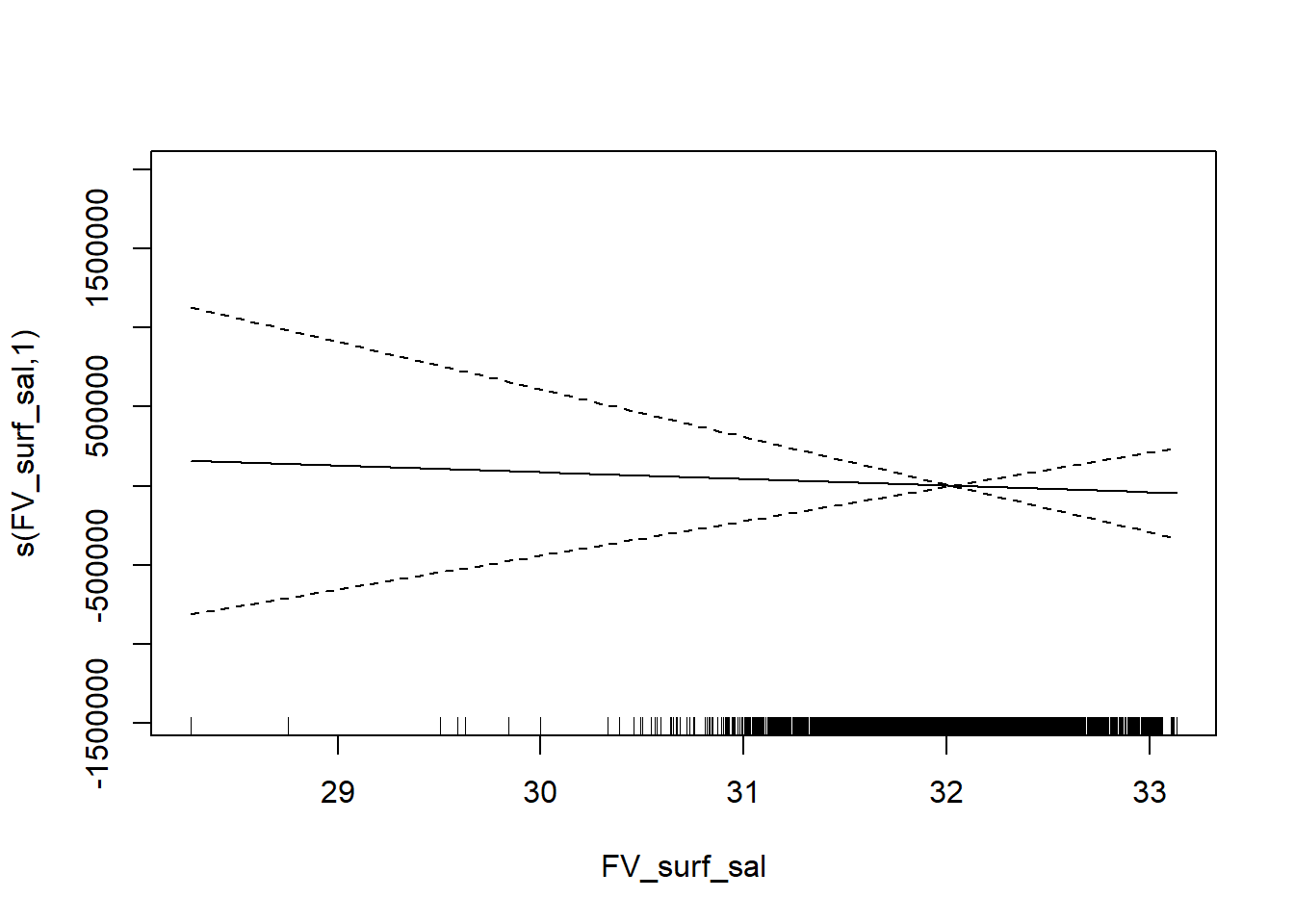
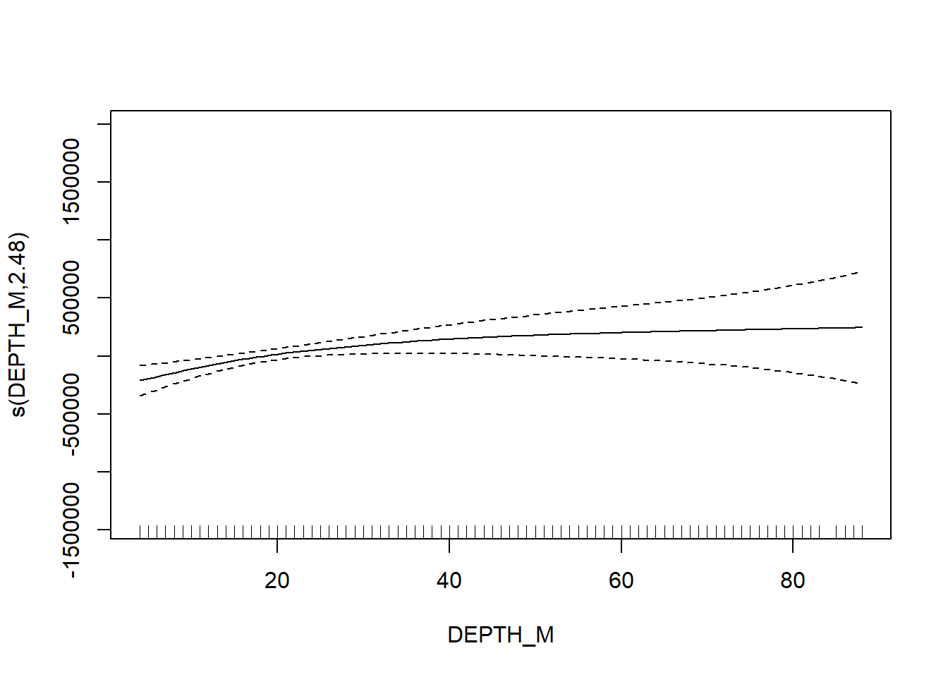
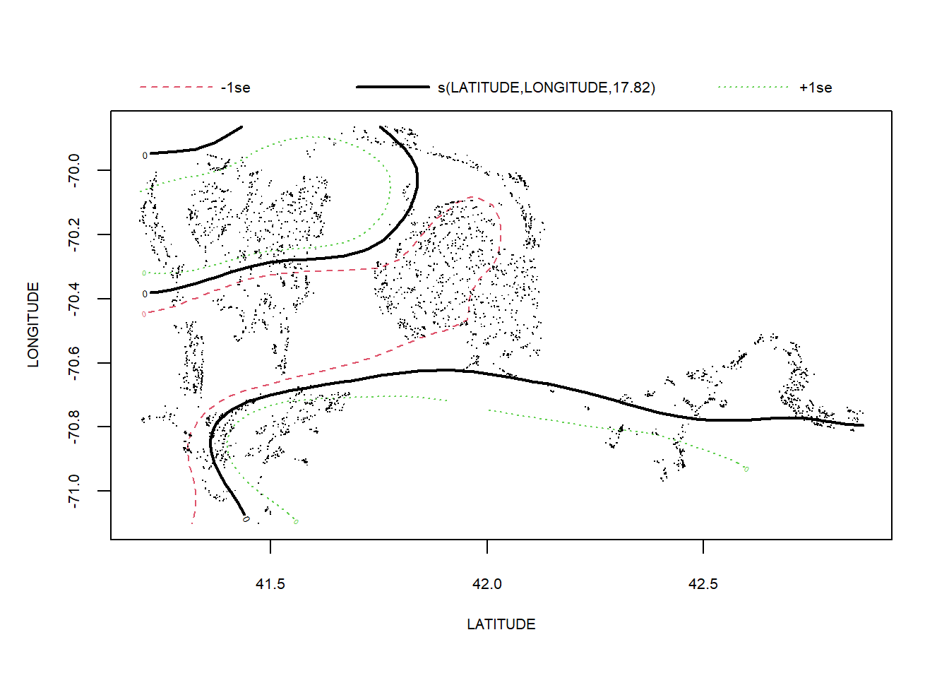
Taxonomic distinctness
# tax distinctness
FV_MA_delta_star_FL <- gamm4(delta_star ~ s(FV_bot_temp) + s(FV_surf_temp) + s(FV_bot_sal) +  s(FV_surf_sal) +   s(DEPTH_M)+ s(LATITUDE, LONGITUDE) , random = ~ (1|YEAR), data = MA_fall)

gam.check(FV_MA_delta_star_FL$gam)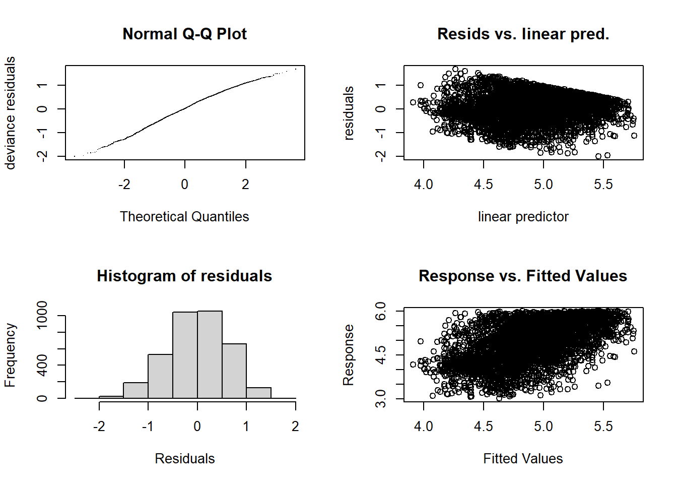
##
## 'gamm' based fit - care required with interpretation.
## Checks based on working residuals may be misleading.
## Basis dimension (k) checking results. Low p-value (k-index<1) may
## indicate that k is too low, especially if edf is close to k'.
##
##                          k'   edf k-index p-value
## s(FV_bot_temp)         9.00  7.10    1.00   0.560
## s(FV_surf_temp)        9.00  4.85    0.99   0.220
## s(FV_bot_sal)          9.00  1.00    0.95   0.005 **
## s(FV_surf_sal)         9.00  1.00    0.99   0.290
## s(DEPTH_M)             9.00  3.80    0.91  <2e-16 ***
## s(LATITUDE,LONGITUDE) 29.00 24.31    0.95  <2e-16 ***
## ---
## Signif. codes: 0 '***' 0.001 '**' 0.01 '*' 0.05 '.' 0.1 ' ' 1summary(FV_MA_delta_star_FL$gam)##
## Family: gaussian
## Link function: identity
##
## Formula:
## delta_star ~ s(FV_bot_temp) + s(FV_surf_temp) + s(FV_bot_sal) +
## s(FV_surf_sal) + s(DEPTH_M) + s(LATITUDE, LONGITUDE)
##
## Parametric coefficients:
## Estimate Std. Error t value Pr(>|t|)
## (Intercept) 4.88882 0.02734 178.8 <2e-16 ***
## ---
## Signif. codes: 0 '***' 0.001 '**' 0.01 '*' 0.05 '.' 0.1 ' ' 1
##
## Approximate significance of smooth terms:
## edf Ref.df F p-value
## s(FV_bot_temp) 7.099 7.099 17.531 < 2e-16 ***
## s(FV_surf_temp) 4.854 4.854 5.823 2.75e-05 ***
## s(FV_bot_sal) 1.000 1.000 12.383 0.000438 ***
## s(FV_surf_sal) 1.000 1.000 4.918 0.026647 *
## s(DEPTH_M) 3.802 3.802 10.309 2.77e-07 ***
## s(LATITUDE,LONGITUDE) 24.307 24.307 9.257 < 2e-16 ***
## ---
## Signif. codes: 0 '***' 0.001 '**' 0.01 '*' 0.05 '.' 0.1 ' ' 1
##
## R-sq.(adj) = 0.26
## lmer.REML = 6580.3 Scale est. = 0.33751 n = 3630plot(FV_MA_delta_star_FL$gam)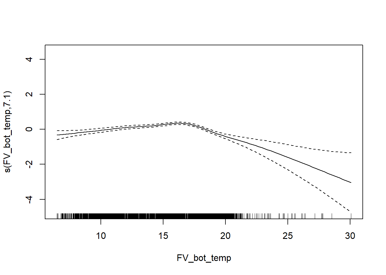
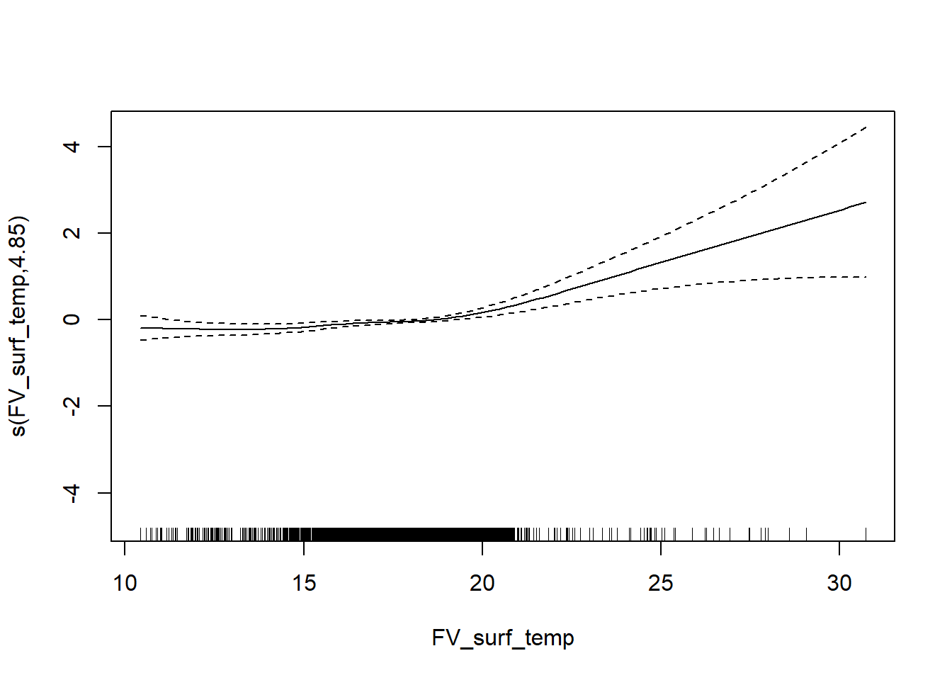
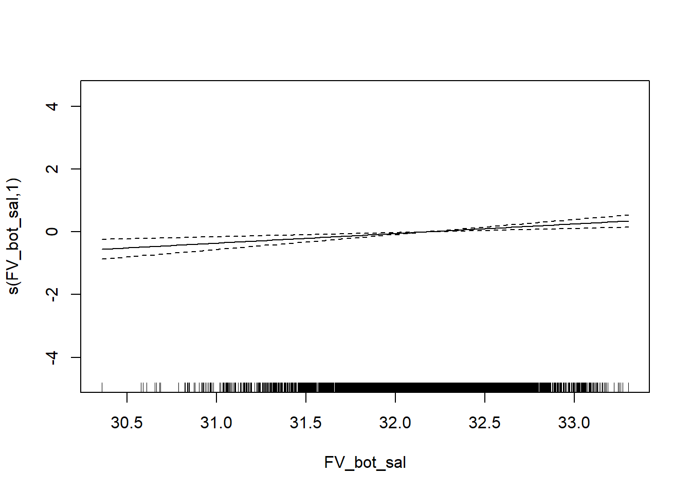
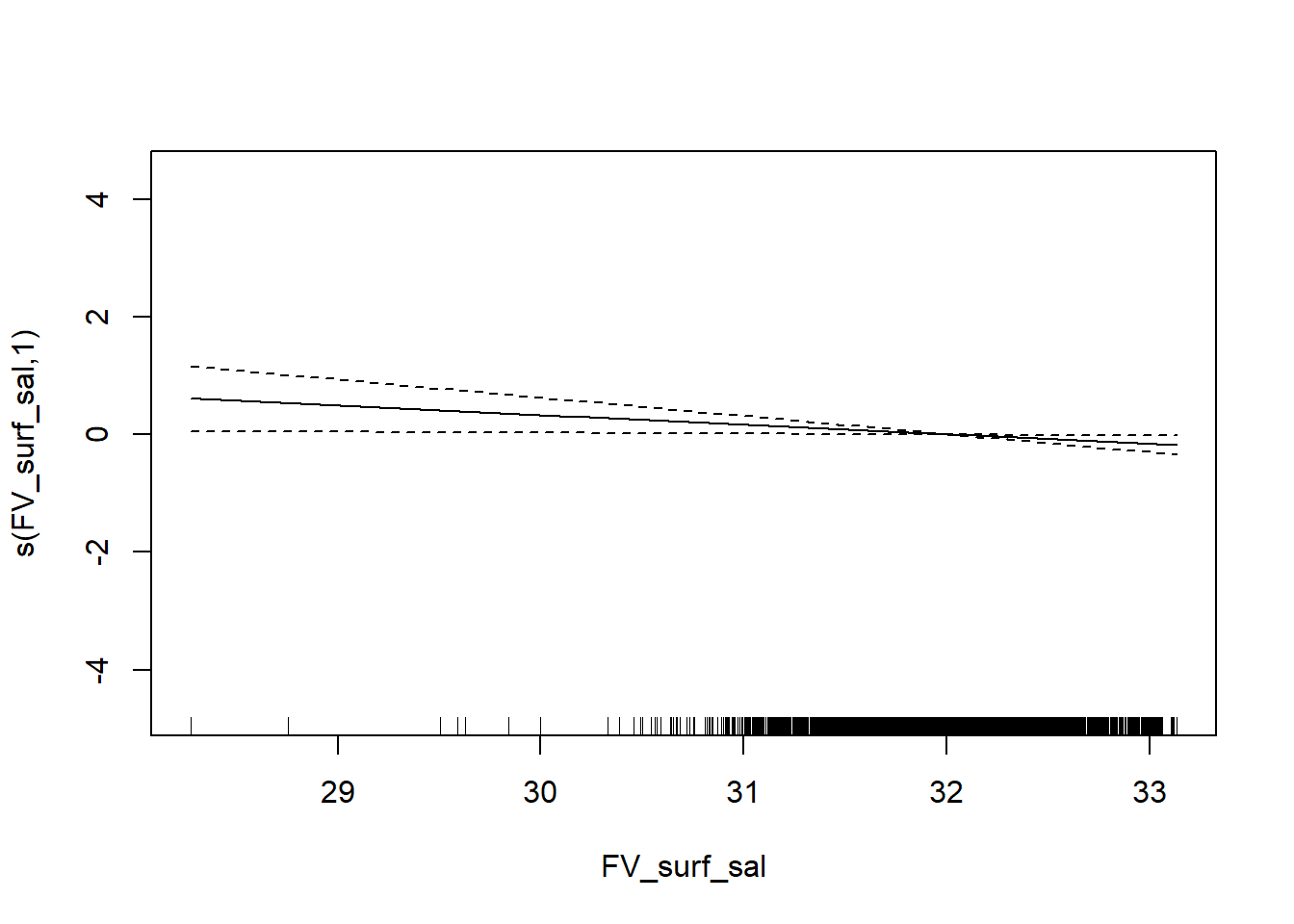
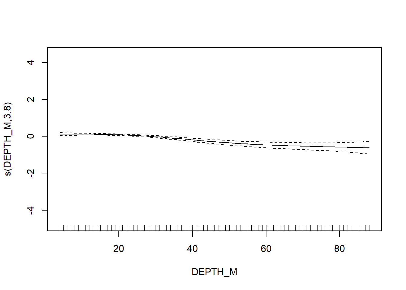
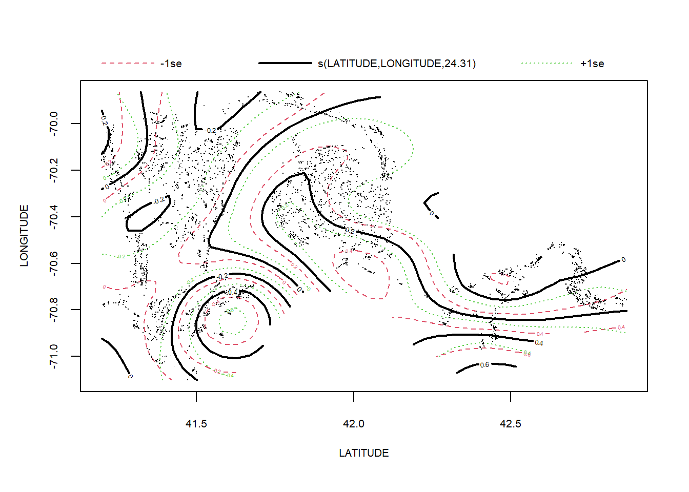
Average taxonomic distinctness
# avg tax distinctness
FV_MA_delta_plus_FL <- gamm4(delta_plus ~ s(FV_bot_temp) + s(FV_surf_temp) + s(FV_bot_sal) +  s(FV_surf_sal) +  s(DEPTH_M)+ s(LATITUDE, LONGITUDE) , random = ~ (1|YEAR), data = MA_fall)

gam.check(FV_MA_delta_plus_FL$gam)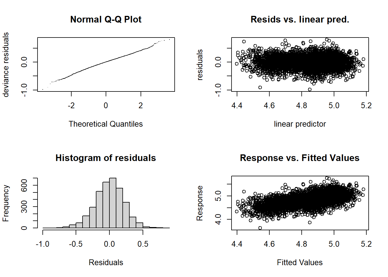
##
## 'gamm' based fit - care required with interpretation.
## Checks based on working residuals may be misleading.
## Basis dimension (k) checking results. Low p-value (k-index<1) may
## indicate that k is too low, especially if edf is close to k'.
##
##                          k'   edf k-index p-value
## s(FV_bot_temp)         9.00  7.40    1.00    0.48
## s(FV_surf_temp)        9.00  3.62    0.98    0.12
## s(FV_bot_sal)          9.00  1.00    1.00    0.48
## s(FV_surf_sal)         9.00  3.58    0.98    0.13
## s(DEPTH_M)             9.00  7.07    0.90  <2e-16 ***
## s(LATITUDE,LONGITUDE) 29.00 27.40    0.91  <2e-16 ***
## ---
## Signif. codes: 0 '***' 0.001 '**' 0.01 '*' 0.05 '.' 0.1 ' ' 1summary(FV_MA_delta_plus_FL$gam)##
## Family: gaussian
## Link function: identity
##
## Formula:
## delta_plus ~ s(FV_bot_temp) + s(FV_surf_temp) + s(FV_bot_sal) +
## s(FV_surf_sal) + s(DEPTH_M) + s(LATITUDE, LONGITUDE)
##
## Parametric coefficients:
## Estimate Std. Error t value Pr(>|t|)
## (Intercept) 4.845865 0.008204 590.7 <2e-16 ***
## ---
## Signif. codes: 0 '***' 0.001 '**' 0.01 '*' 0.05 '.' 0.1 ' ' 1
##
## Approximate significance of smooth terms:
## edf Ref.df F p-value
## s(FV_bot_temp) 7.402 7.402 11.285 < 2e-16 ***
## s(FV_surf_temp) 3.615 3.615 11.189 1.62e-07 ***
## s(FV_bot_sal) 1.000 1.000 20.806 5.91e-06 ***
## s(FV_surf_sal) 3.583 3.583 3.996 0.00601 **
## s(DEPTH_M) 7.067 7.067 18.593 < 2e-16 ***
## s(LATITUDE,LONGITUDE) 27.405 27.405 21.370 < 2e-16 ***
## ---
## Signif. codes: 0 '***' 0.001 '**' 0.01 '*' 0.05 '.' 0.1 ' ' 1
##
## R-sq.(adj) = 0.336
## lmer.REML = -628.87 Scale est. = 0.04571 n = 3635plot(FV_MA_delta_plus_FL$gam)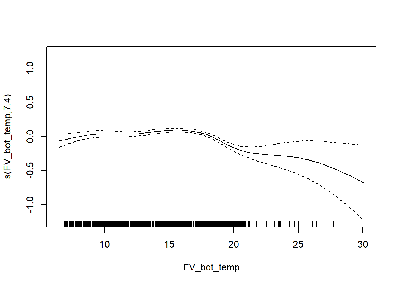
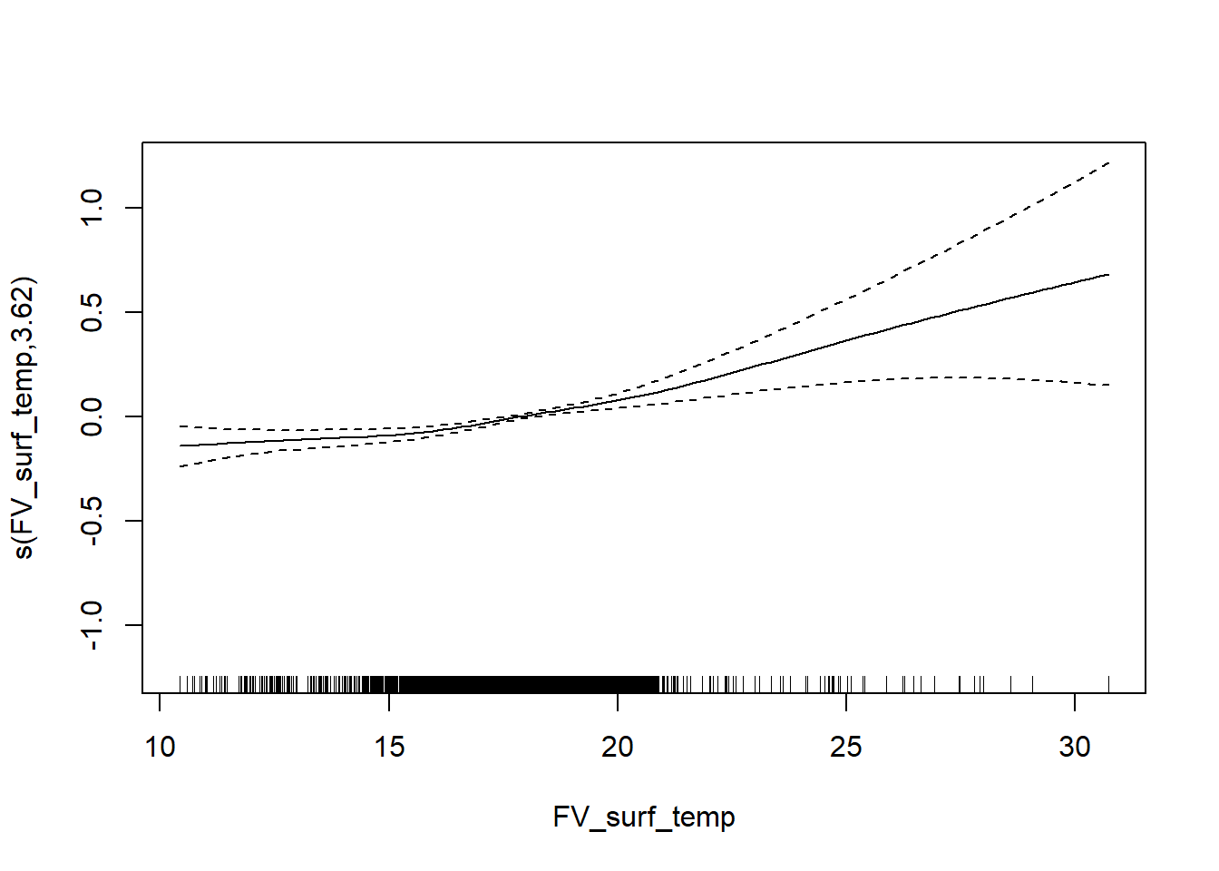
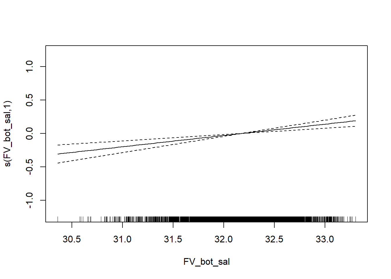
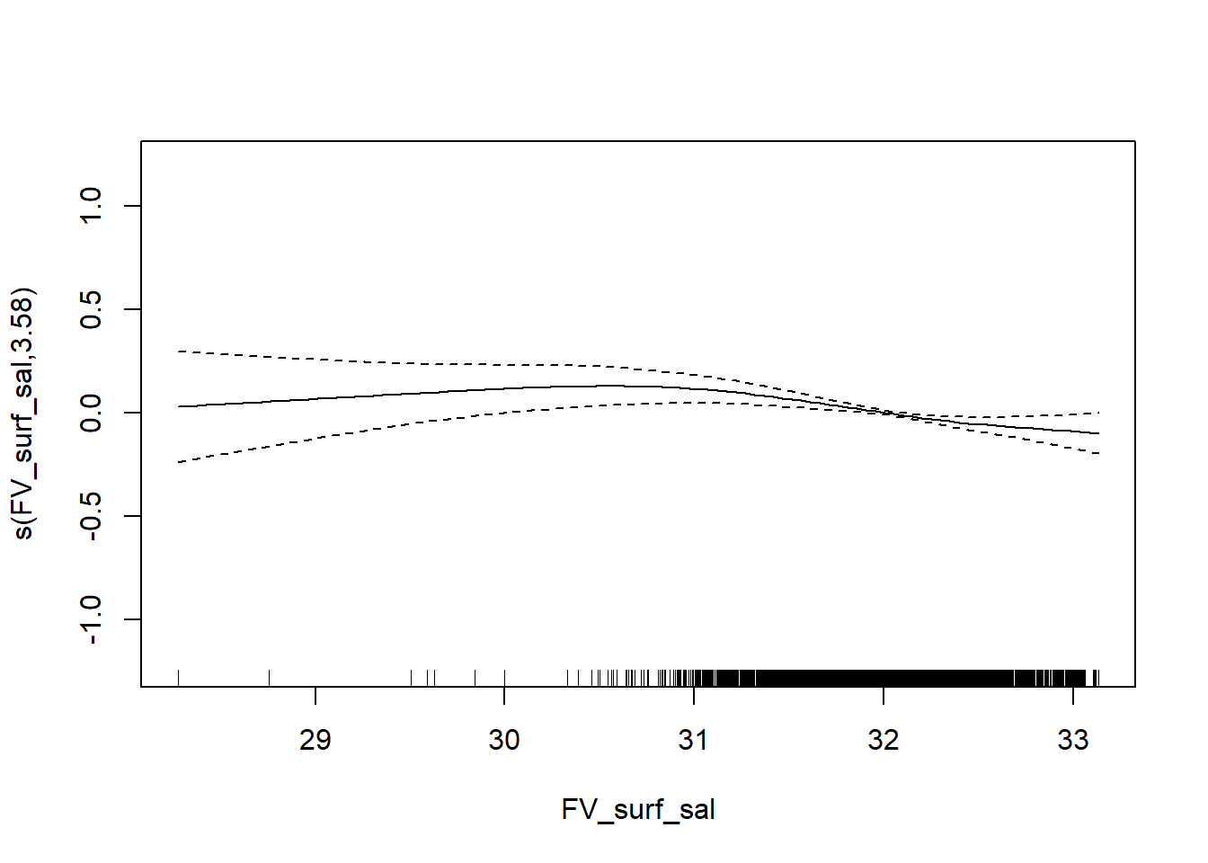
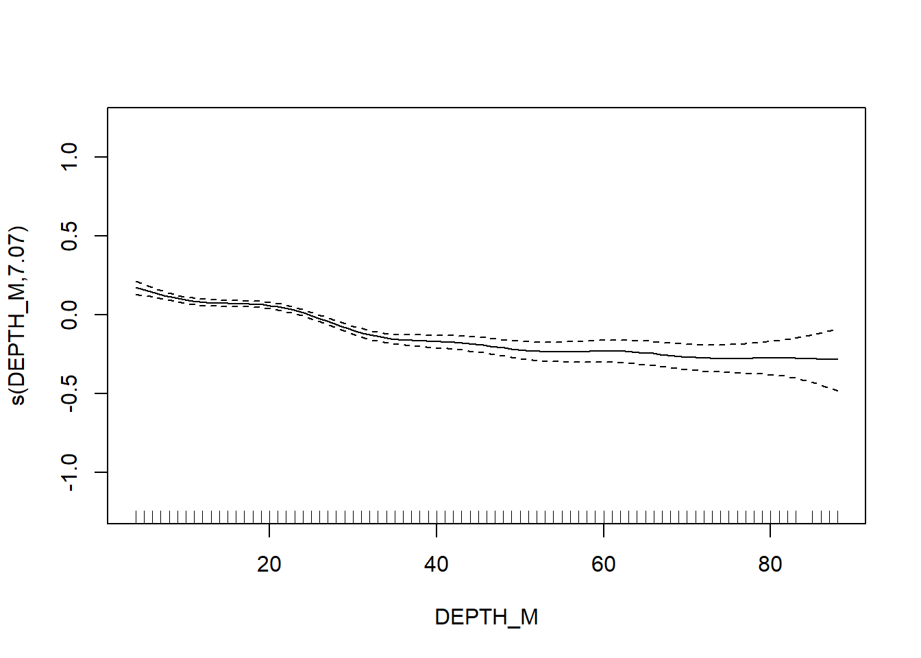
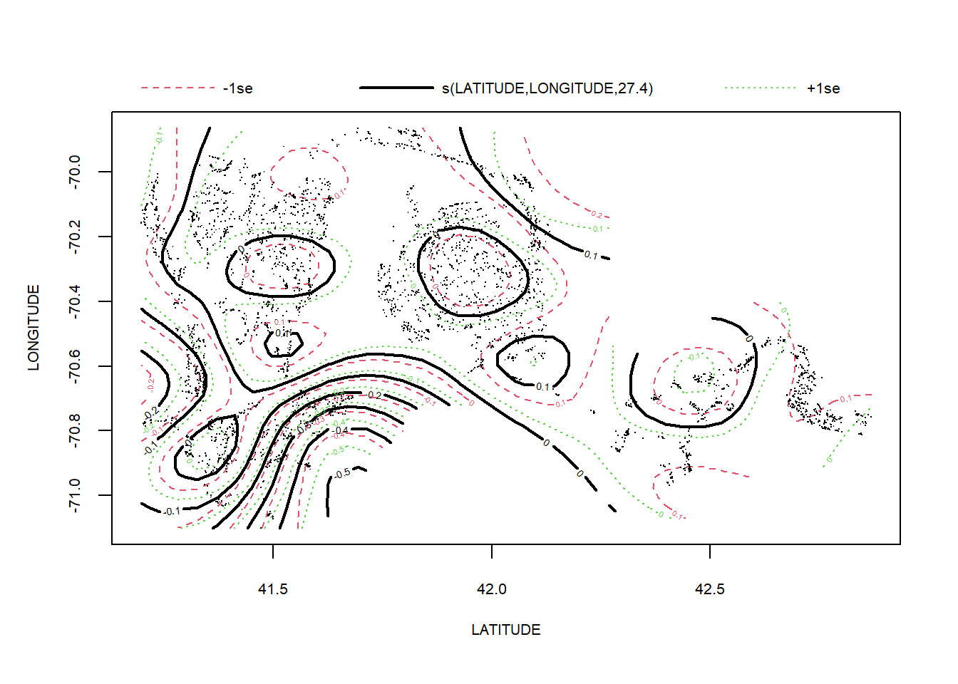
Variation in taxonomic distinctness
# var in tax distinctness
FV_MA_delta_var_FL <- gamm4(delta_var ~ s(FV_bot_temp) + s(FV_surf_temp) + s(FV_bot_sal) +  s(FV_surf_sal) +  s(DEPTH_M)+ s(LATITUDE, LONGITUDE) , random = ~ (1|YEAR), data = MA_fall)

gam.check(FV_MA_delta_var_FL$gam)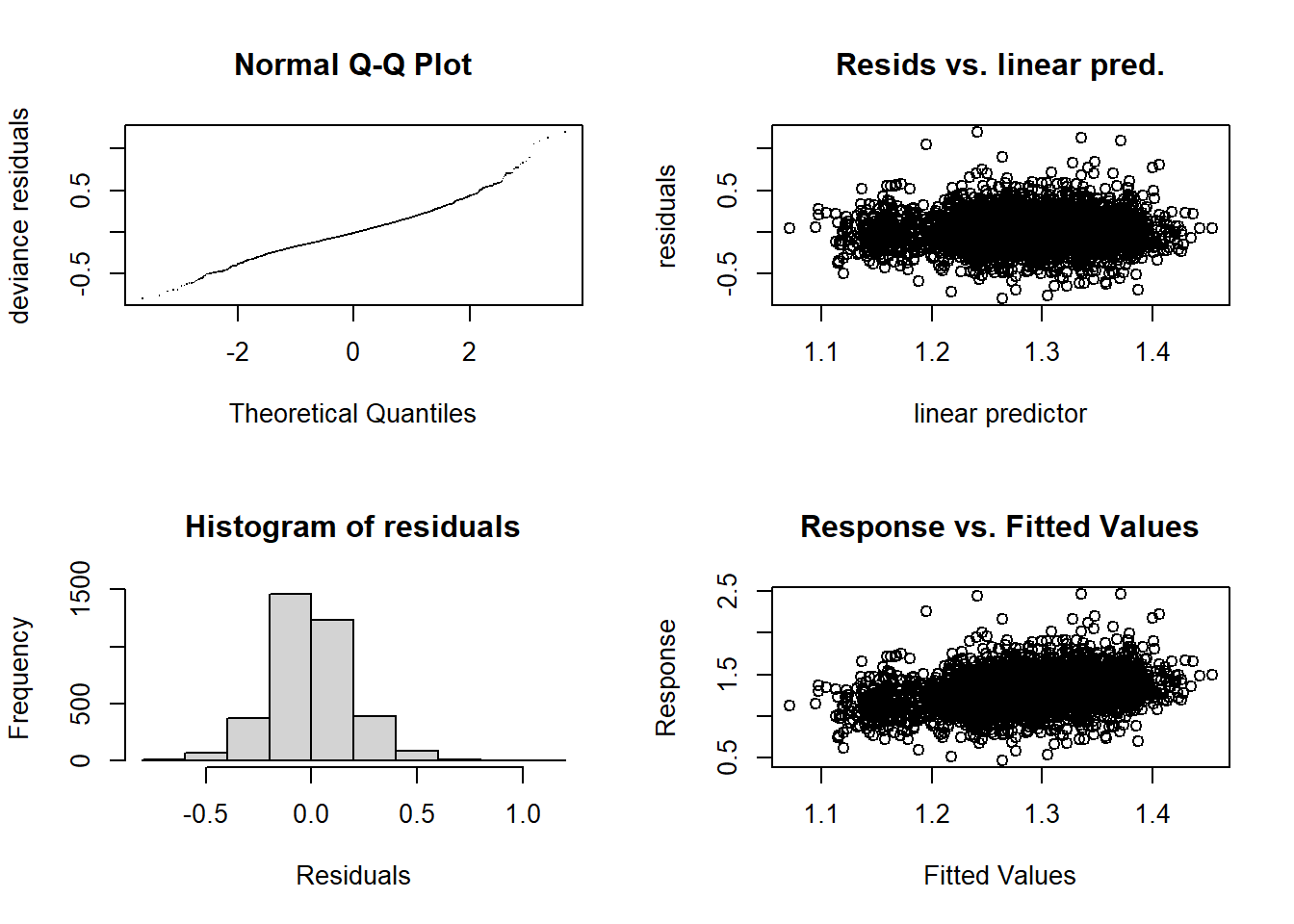
##
## 'gamm' based fit - care required with interpretation.
## Checks based on working residuals may be misleading.
## Basis dimension (k) checking results. Low p-value (k-index<1) may
## indicate that k is too low, especially if edf is close to k'.
##
##                          k'   edf k-index p-value
## s(FV_bot_temp)         9.00  5.57    0.98   0.110
## s(FV_surf_temp)        9.00  1.00    1.01   0.620
## s(FV_bot_sal)          9.00  1.00    0.98   0.145
## s(FV_surf_sal)         9.00  3.93    0.97   0.015 *
## s(DEPTH_M)             9.00  1.00    0.96  <2e-16 ***
## s(LATITUDE,LONGITUDE) 29.00 22.82    0.95  <2e-16 ***
## ---
## Signif. codes: 0 '***' 0.001 '**' 0.01 '*' 0.05 '.' 0.1 ' ' 1summary(FV_MA_delta_var_FL$gam)##
## Family: gaussian
## Link function: identity
##
## Formula:
## delta_var ~ s(FV_bot_temp) + s(FV_surf_temp) + s(FV_bot_sal) +
## s(FV_surf_sal) + s(DEPTH_M) + s(LATITUDE, LONGITUDE)
##
## Parametric coefficients:
## Estimate Std. Error t value Pr(>|t|)
## (Intercept) 1.285889 0.006556 196.1 <2e-16 ***
## ---
## Signif. codes: 0 '***' 0.001 '**' 0.01 '*' 0.05 '.' 0.1 ' ' 1
##
## Approximate significance of smooth terms:
## edf Ref.df F p-value
## s(FV_bot_temp) 5.571 5.571 3.539 0.00197 **
## s(FV_surf_temp) 1.000 1.000 4.540 0.03318 *
## s(FV_bot_sal) 1.000 1.000 0.291 0.58967
## s(FV_surf_sal) 3.926 3.926 1.366 0.23957
## s(DEPTH_M) 1.000 1.000 1.132 0.28738
## s(LATITUDE,LONGITUDE) 22.823 22.823 7.802 < 2e-16 ***
## ---
## Signif. codes: 0 '***' 0.001 '**' 0.01 '*' 0.05 '.' 0.1 ' ' 1
##
## R-sq.(adj) = 0.0881
## lmer.REML = -1345.6 Scale est. = 0.038411 n = 3635plot(FV_MA_delta_var_FL$gam)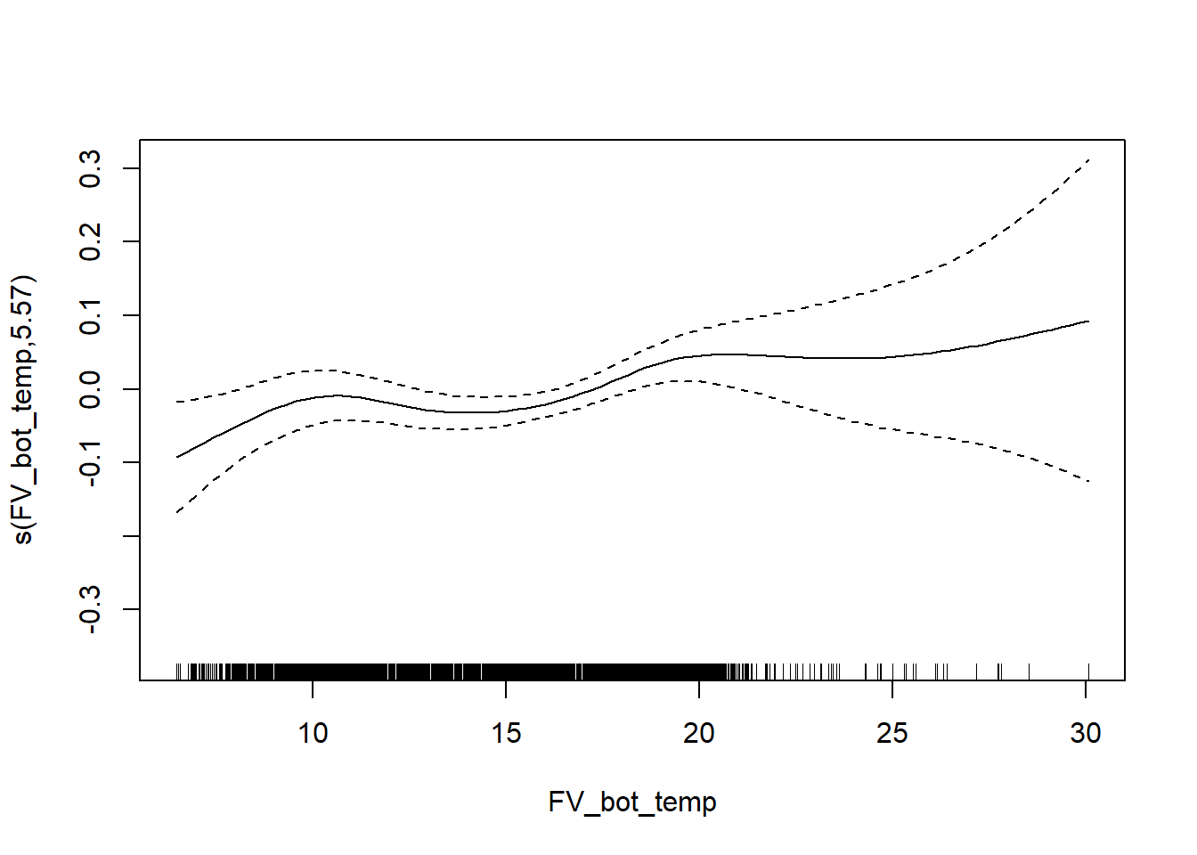
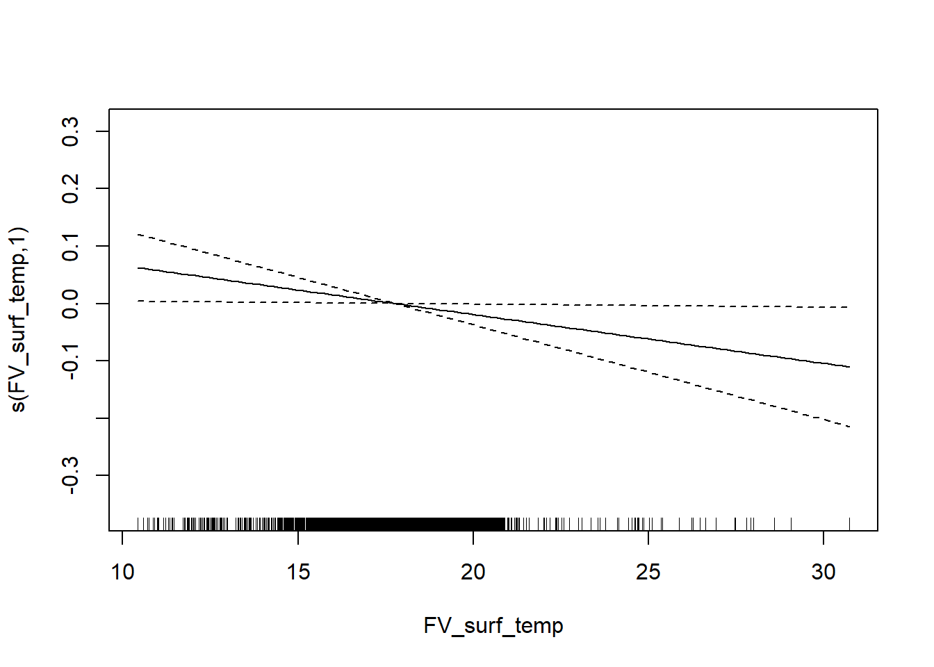
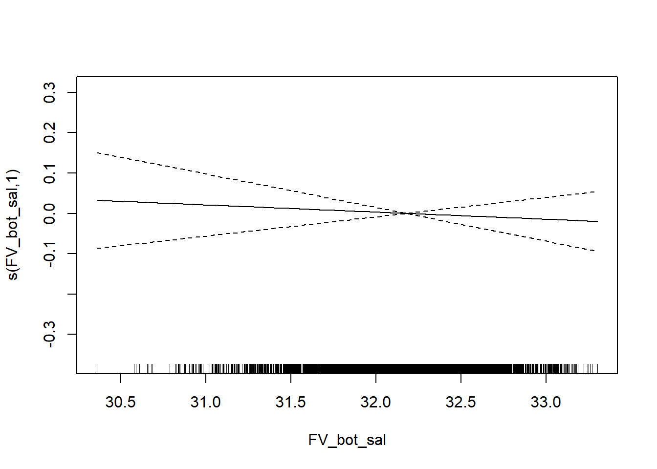
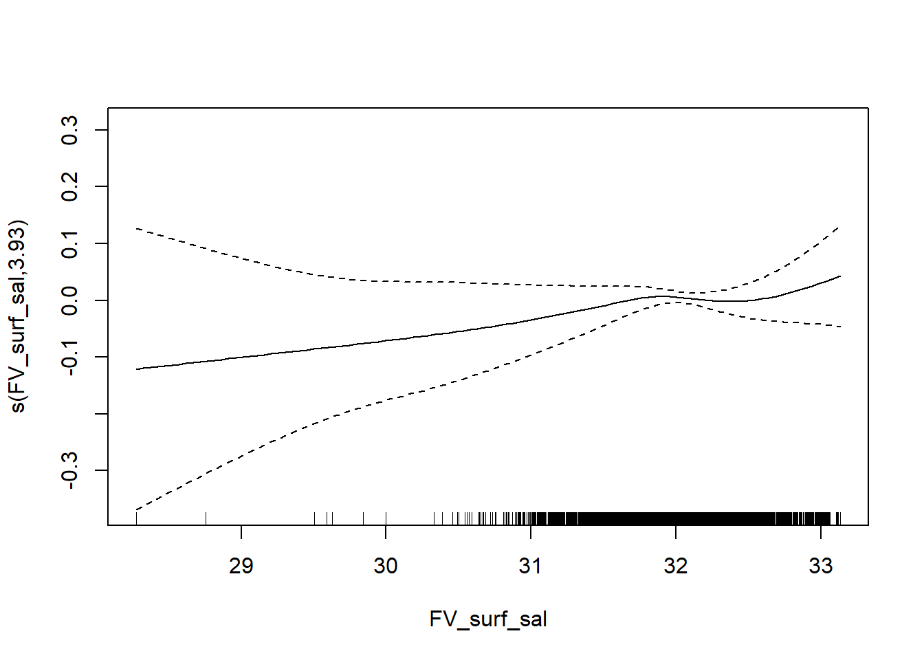
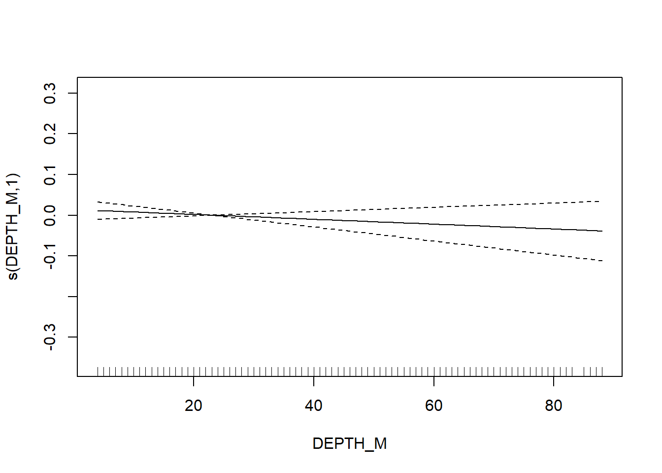
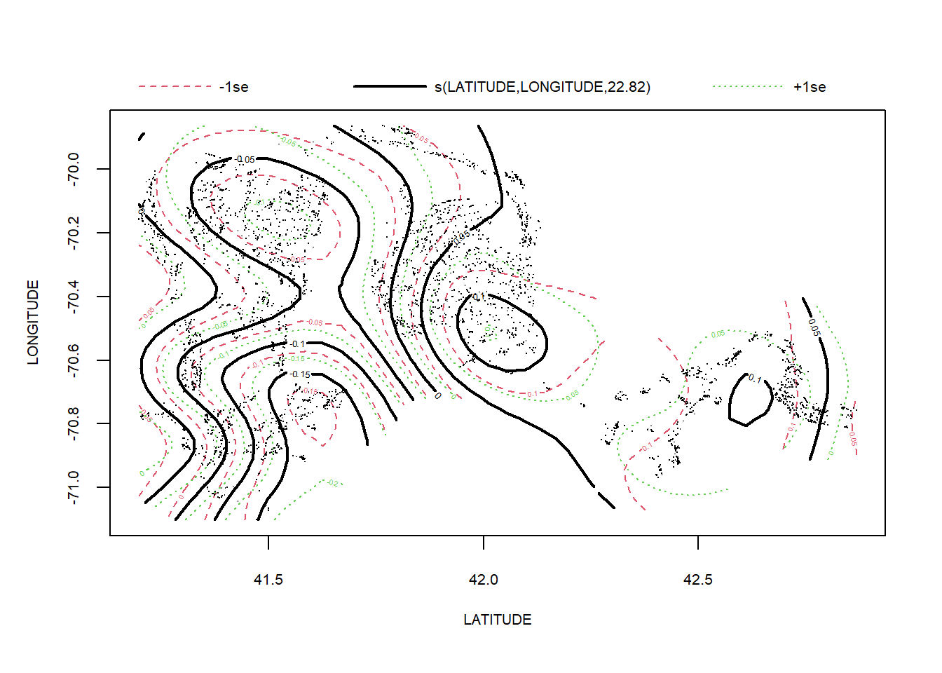
MADMF spring GAMMs
Species richness
# number of species
FV_MA_N_SP <- gamm4(N_species ~ s(FV_bot_temp) + s(FV_surf_temp) + s(FV_bot_sal) +  s(FV_surf_sal) +   s(DEPTH_M)+ s(LATITUDE, LONGITUDE) , random = ~ (1|YEAR), data = MA_spring)

gam.check(FV_MA_N_SP$gam)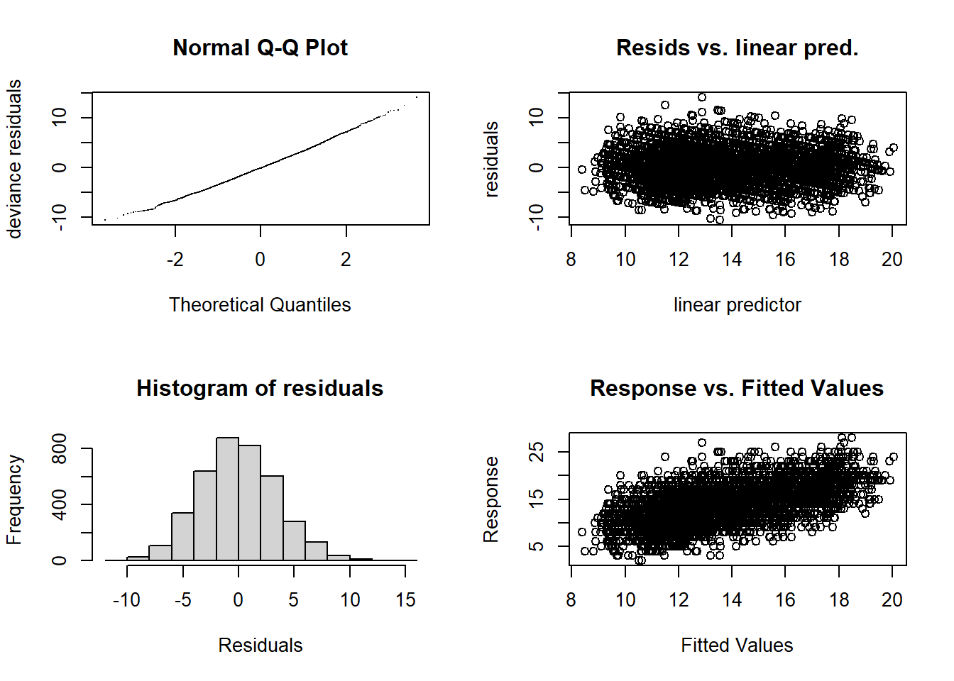
##
## 'gamm' based fit - care required with interpretation.
## Checks based on working residuals may be misleading.
## Basis dimension (k) checking results. Low p-value (k-index<1) may
## indicate that k is too low, especially if edf is close to k'.
##
##                          k'   edf k-index p-value
## s(FV_bot_temp)         9.00  4.51    0.98   0.130
## s(FV_surf_temp)        9.00  1.00    0.98   0.065 .
## s(FV_bot_sal)          9.00  3.00    1.00   0.510
## s(FV_surf_sal)         9.00  1.00    0.98   0.190
## s(DEPTH_M)             9.00  4.80    0.89  <2e-16 ***
## s(LATITUDE,LONGITUDE) 29.00 26.32    0.87  <2e-16 ***
## ---
## Signif. codes: 0 '***' 0.001 '**' 0.01 '*' 0.05 '.' 0.1 ' ' 1summary(FV_MA_N_SP$gam)##
## Family: gaussian
## Link function: identity
##
## Formula:
## N_species ~ s(FV_bot_temp) + s(FV_surf_temp) + s(FV_bot_sal) +
## s(FV_surf_sal) + s(DEPTH_M) + s(LATITUDE, LONGITUDE)
##
## Parametric coefficients:
## Estimate Std. Error t value Pr(>|t|)
## (Intercept) 13.7601 0.2051 67.1 <2e-16 ***
## ---
## Signif. codes: 0 '***' 0.001 '**' 0.01 '*' 0.05 '.' 0.1 ' ' 1
##
## Approximate significance of smooth terms:
## edf Ref.df F p-value
## s(FV_bot_temp) 4.506 4.506 5.367 0.00015 ***
## s(FV_surf_temp) 1.000 1.000 1.925 0.16534
## s(FV_bot_sal) 3.005 3.005 3.112 0.02426 *
## s(FV_surf_sal) 1.000 1.000 5.768 0.01637 *
## s(DEPTH_M) 4.798 4.798 47.362 < 2e-16 ***
## s(LATITUDE,LONGITUDE) 26.320 26.320 23.225 < 2e-16 ***
## ---
## Signif. codes: 0 '***' 0.001 '**' 0.01 '*' 0.05 '.' 0.1 ' ' 1
##
## R-sq.(adj) = 0.342
## lmer.REML = 20245 Scale est. = 10.235 n = 3877plot(FV_MA_N_SP$gam)
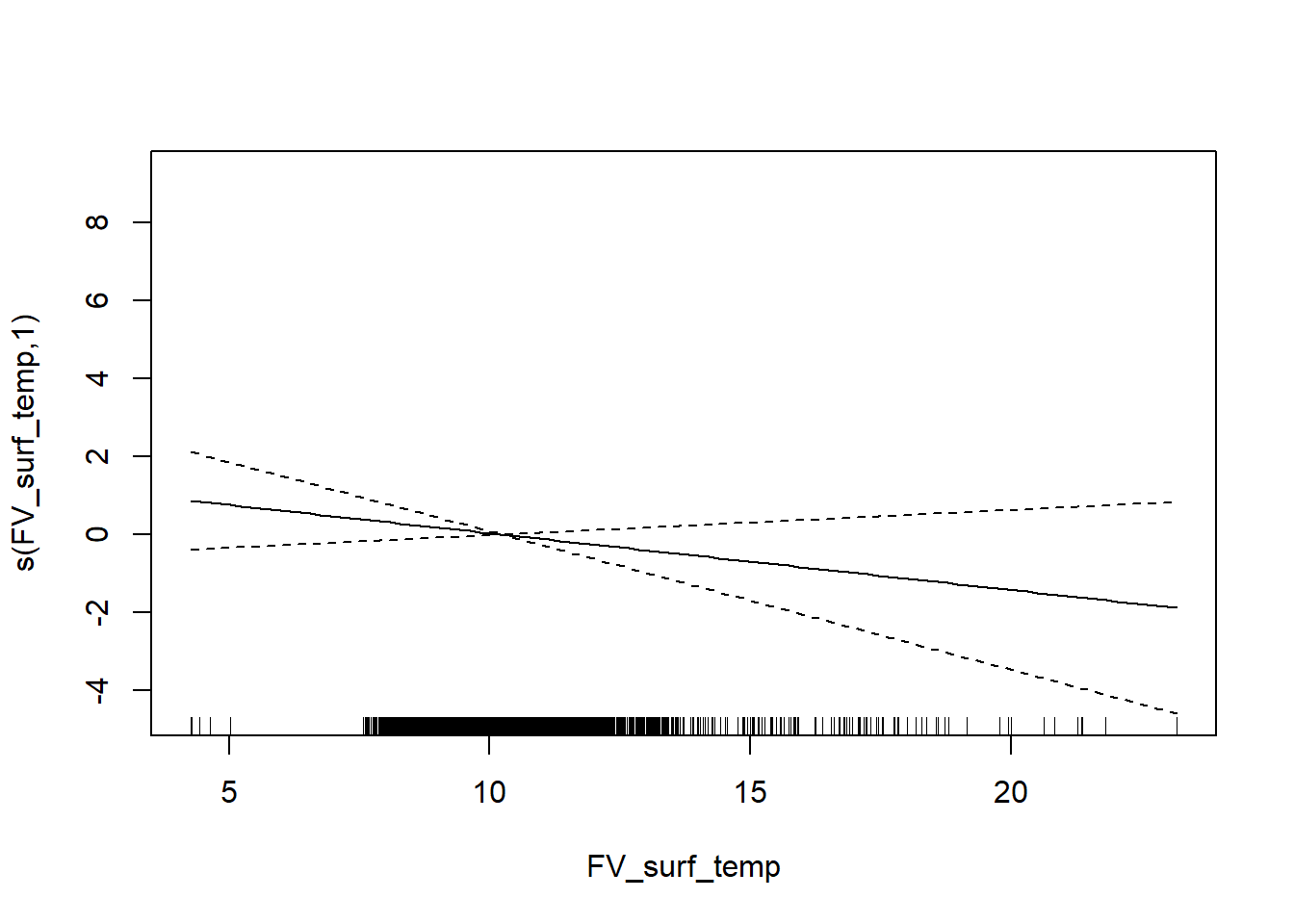


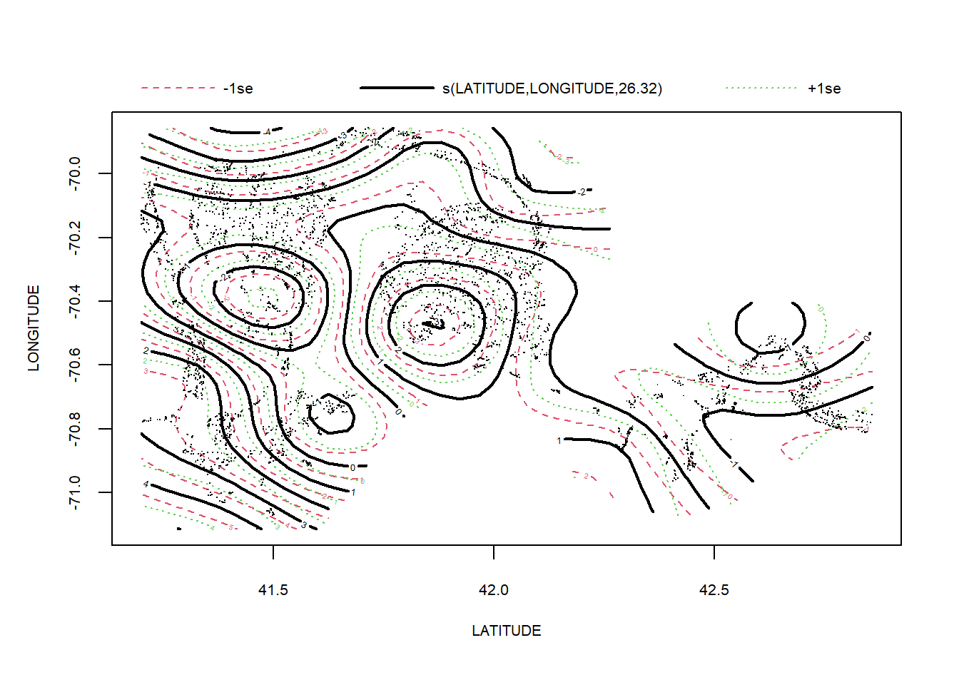
Shannon-Weiner diversity
# S-W
FV_MA_H_SP <- gamm4(H_index ~ s(FV_bot_temp) + s(FV_surf_temp) + s(FV_bot_sal) +  s(FV_surf_sal) +  s(DEPTH_M)+ s(LATITUDE, LONGITUDE) , random = ~ (1|YEAR), data = MA_spring)

gam.check(FV_MA_H_SP$gam)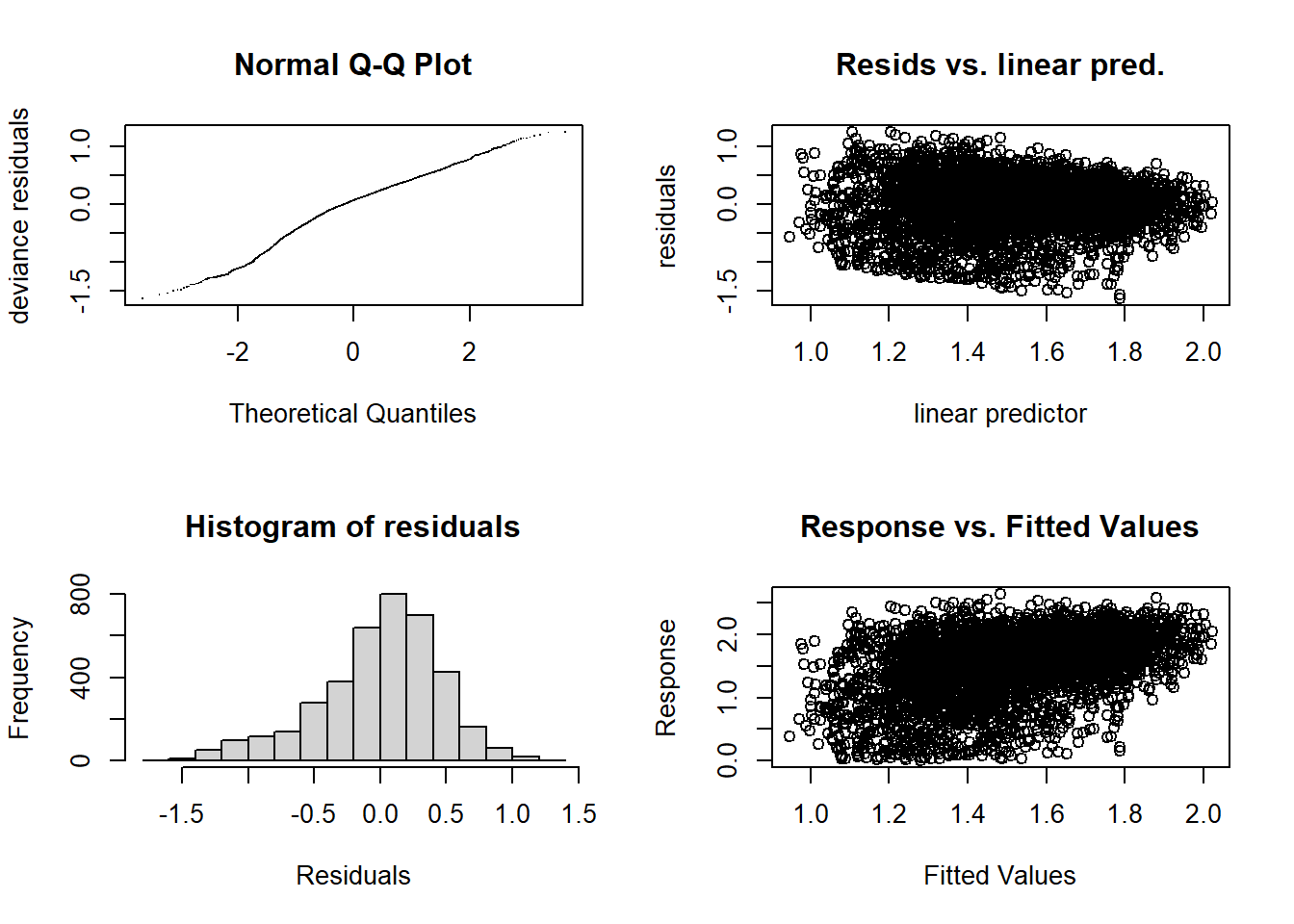
##
## 'gamm' based fit - care required with interpretation.
## Checks based on working residuals may be misleading.
## Basis dimension (k) checking results. Low p-value (k-index<1) may
## indicate that k is too low, especially if edf is close to k'.
##
##                          k'   edf k-index p-value
## s(FV_bot_temp)         9.00  4.88    1.00    0.57
## s(FV_surf_temp)        9.00  1.99    0.99    0.19
## s(FV_bot_sal)          9.00  1.00    1.00    0.43
## s(FV_surf_sal)         9.00  1.00    0.99    0.23
## s(DEPTH_M)             9.00  4.88    0.92  <2e-16 ***
## s(LATITUDE,LONGITUDE) 29.00 25.93    0.95  <2e-16 ***
## ---
## Signif. codes: 0 '***' 0.001 '**' 0.01 '*' 0.05 '.' 0.1 ' ' 1summary(FV_MA_H_SP$gam)##
## Family: gaussian
## Link function: identity
##
## Formula:
## H_index ~ s(FV_bot_temp) + s(FV_surf_temp) + s(FV_bot_sal) +
## s(FV_surf_sal) + s(DEPTH_M) + s(LATITUDE, LONGITUDE)
##
## Parametric coefficients:
## Estimate Std. Error t value Pr(>|t|)
## (Intercept) 1.51614 0.01899 79.84 <2e-16 ***
## ---
## Signif. codes: 0 '***' 0.001 '**' 0.01 '*' 0.05 '.' 0.1 ' ' 1
##
## Approximate significance of smooth terms:
## edf Ref.df F p-value
## s(FV_bot_temp) 4.881 4.881 3.537 0.00278 **
## s(FV_surf_temp) 1.991 1.991 0.294 0.74361
## s(FV_bot_sal) 1.000 1.000 0.014 0.90738
## s(FV_surf_sal) 1.000 1.000 0.015 0.90201
## s(DEPTH_M) 4.883 4.883 14.725 < 2e-16 ***
## s(LATITUDE,LONGITUDE) 25.929 25.929 15.312 < 2e-16 ***
## ---
## Signif. codes: 0 '***' 0.001 '**' 0.01 '*' 0.05 '.' 0.1 ' ' 1
##
## R-sq.(adj) = 0.177
## lmer.REML = 4986.9 Scale est. = 0.20015 n = 3877plot(FV_MA_N_SP$gam)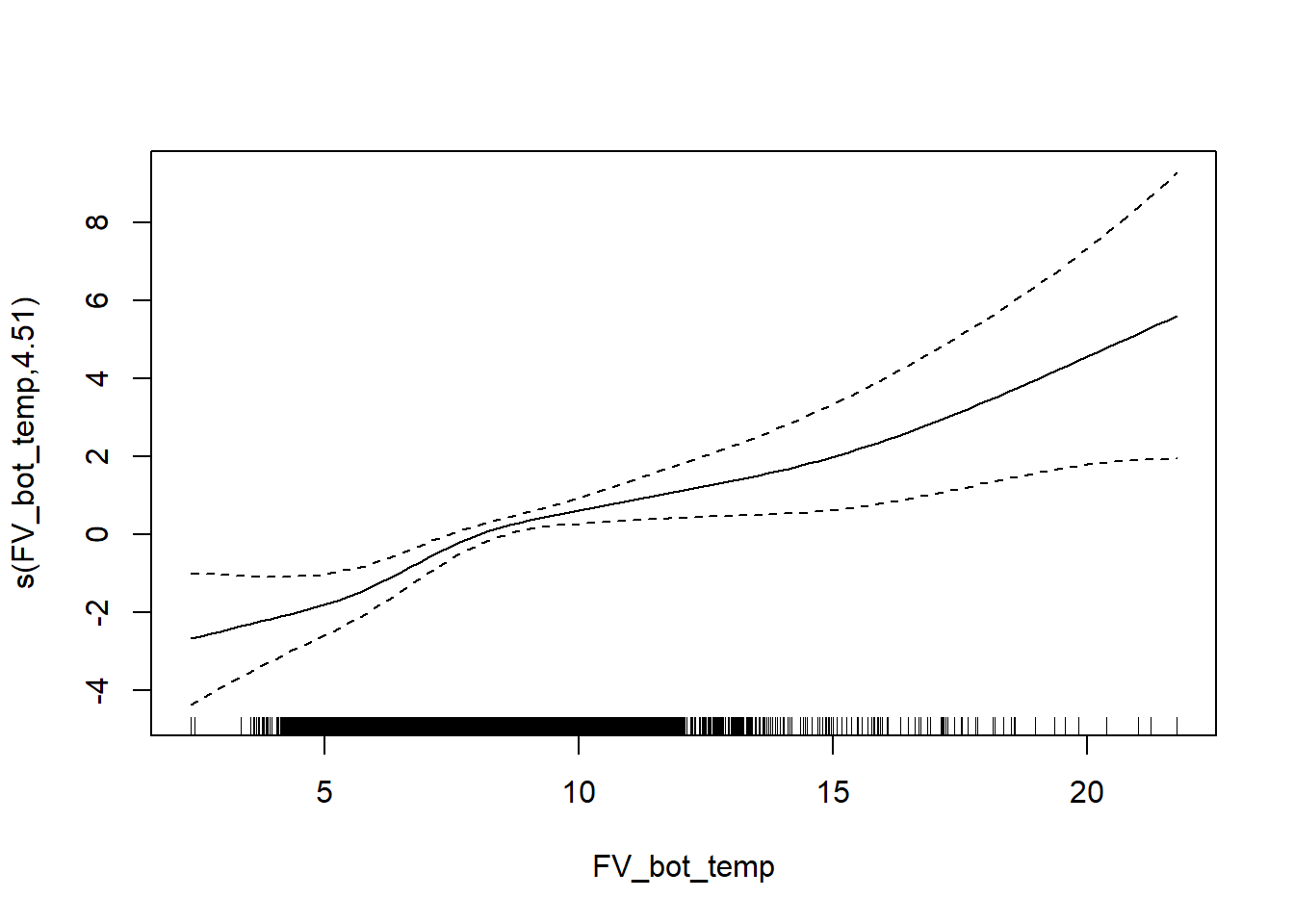

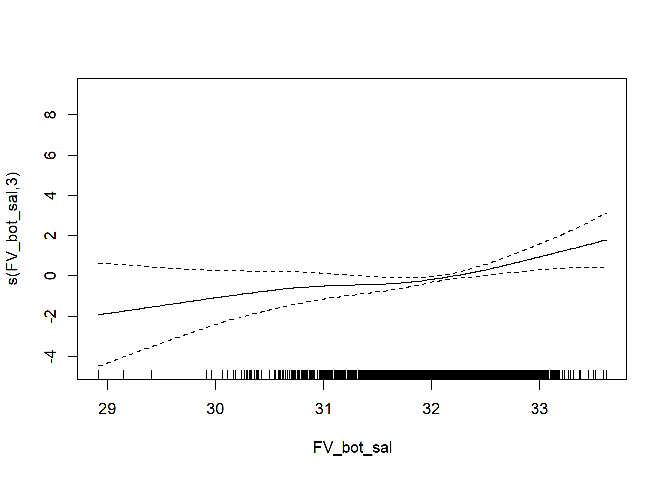
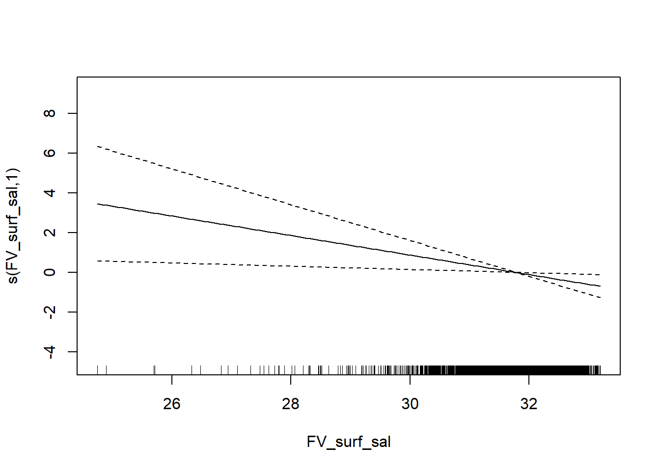
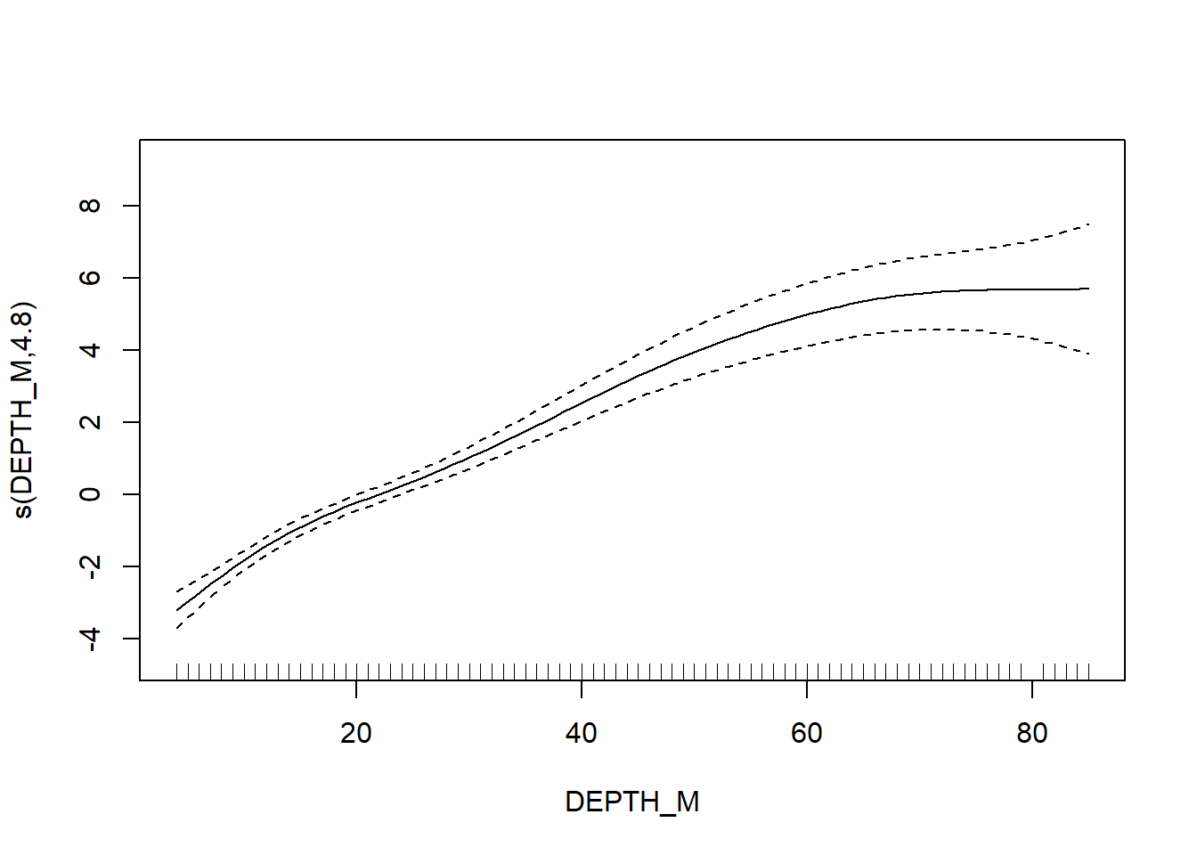

Simpson’s diversity
# Simpsons D
FV_MA_D_SP <- gamm4(D_index ~ s(FV_bot_temp) + s(FV_surf_temp) + s(FV_bot_sal) +  s(FV_surf_sal) +  s(DEPTH_M)+ s(LATITUDE, LONGITUDE) , random = ~ (1|YEAR), data = MA_spring)

gam.check(FV_MA_D_SP$gam)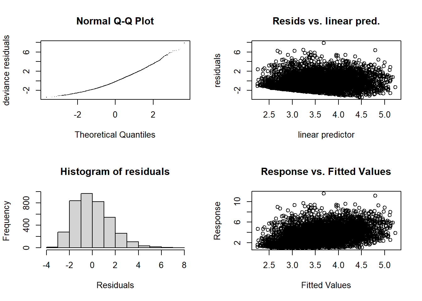
##
## 'gamm' based fit - care required with interpretation.
## Checks based on working residuals may be misleading.
## Basis dimension (k) checking results. Low p-value (k-index<1) may
## indicate that k is too low, especially if edf is close to k'.
##
##                          k'   edf k-index p-value
## s(FV_bot_temp)         9.00  4.48    1.00    0.61
## s(FV_surf_temp)        9.00  1.00    1.00    0.58
## s(FV_bot_sal)          9.00  1.00    1.00    0.49
## s(FV_surf_sal)         9.00  1.00    0.99    0.35
## s(DEPTH_M)             9.00  5.45    0.93  <2e-16 ***
## s(LATITUDE,LONGITUDE) 29.00 24.84    0.97    0.05 *
## ---
## Signif. codes: 0 '***' 0.001 '**' 0.01 '*' 0.05 '.' 0.1 ' ' 1summary(FV_MA_D_SP$gam)##
## Family: gaussian
## Link function: identity
##
## Formula:
## D_index ~ s(FV_bot_temp) + s(FV_surf_temp) + s(FV_bot_sal) +
## s(FV_surf_sal) + s(DEPTH_M) + s(LATITUDE, LONGITUDE)
##
## Parametric coefficients:
## Estimate Std. Error t value Pr(>|t|)
## (Intercept) 3.6568 0.0532 68.74 <2e-16 ***
## ---
## Signif. codes: 0 '***' 0.001 '**' 0.01 '*' 0.05 '.' 0.1 ' ' 1
##
## Approximate significance of smooth terms:
## edf Ref.df F p-value
## s(FV_bot_temp) 4.480 4.480 2.135 0.0452 *
## s(FV_surf_temp) 1.000 1.000 0.013 0.9093
## s(FV_bot_sal) 1.000 1.000 0.821 0.3650
## s(FV_surf_sal) 1.000 1.000 0.103 0.7482
## s(DEPTH_M) 5.447 5.447 10.202 <2e-16 ***
## s(LATITUDE,LONGITUDE) 24.836 24.836 11.526 <2e-16 ***
## ---
## Signif. codes: 0 '***' 0.001 '**' 0.01 '*' 0.05 '.' 0.1 ' ' 1
##
## R-sq.(adj) = 0.131
## lmer.REML = 14546 Scale est. = 2.3839 n = 3877plot(FV_MA_D_SP$gam)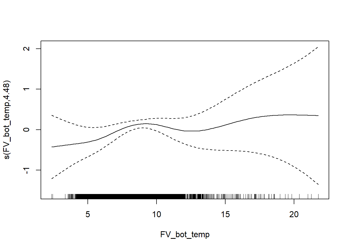
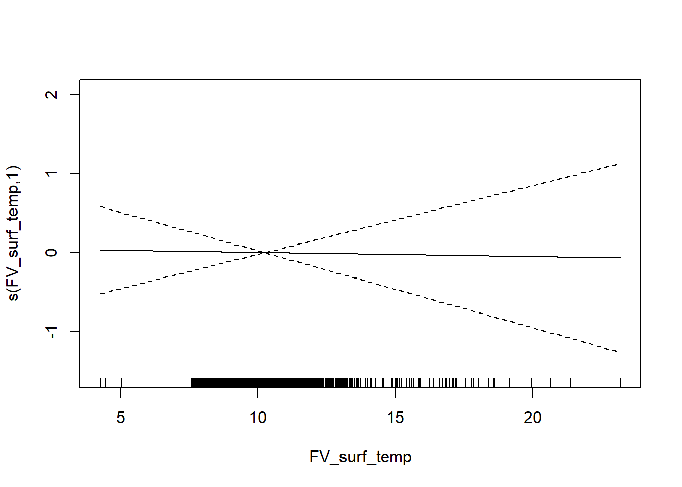
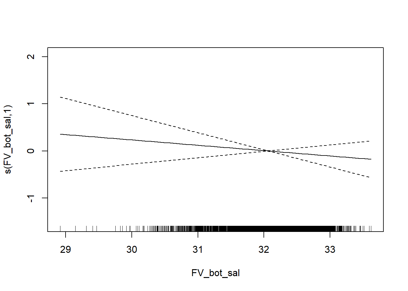
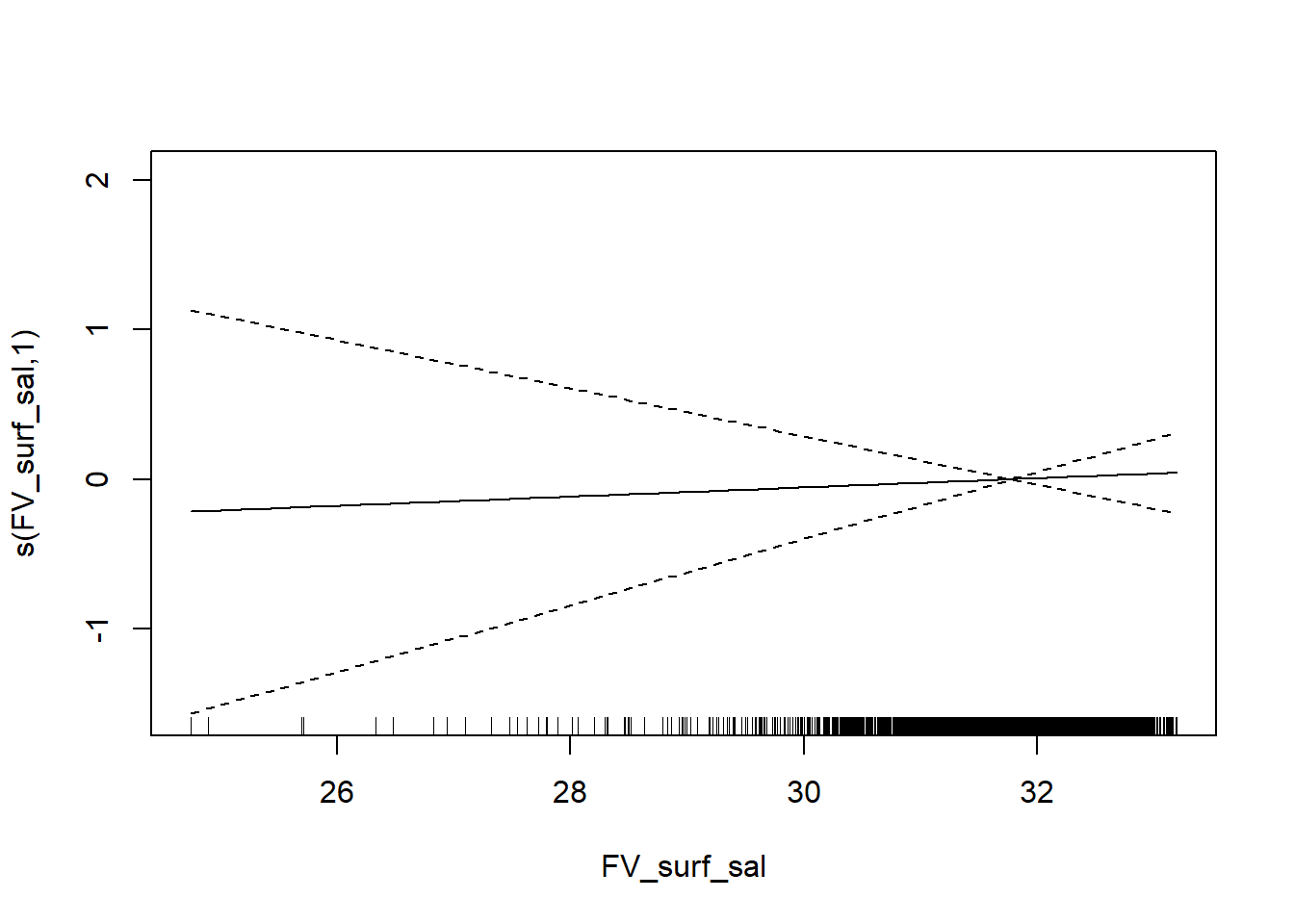
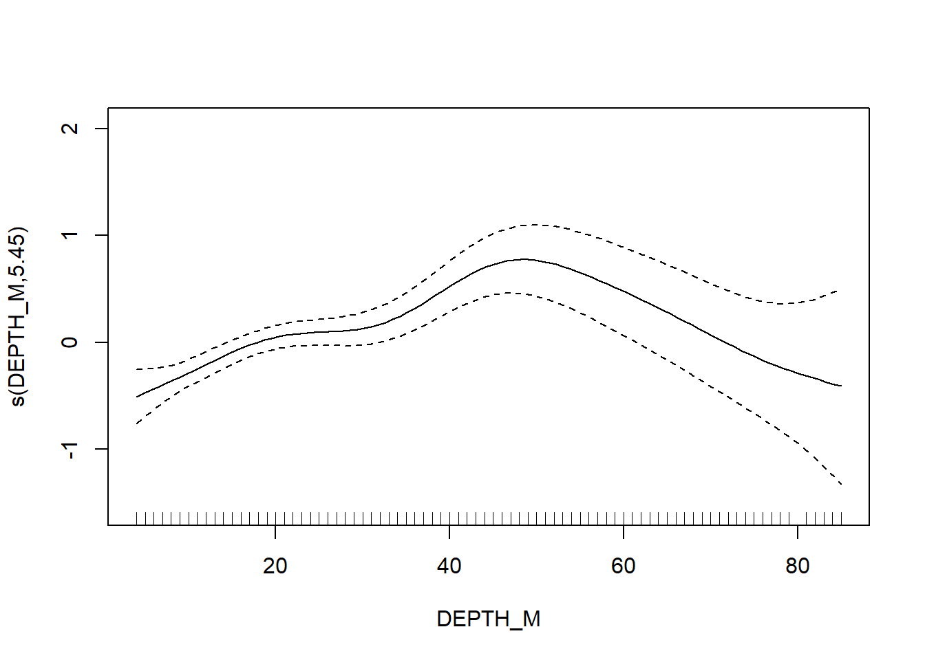
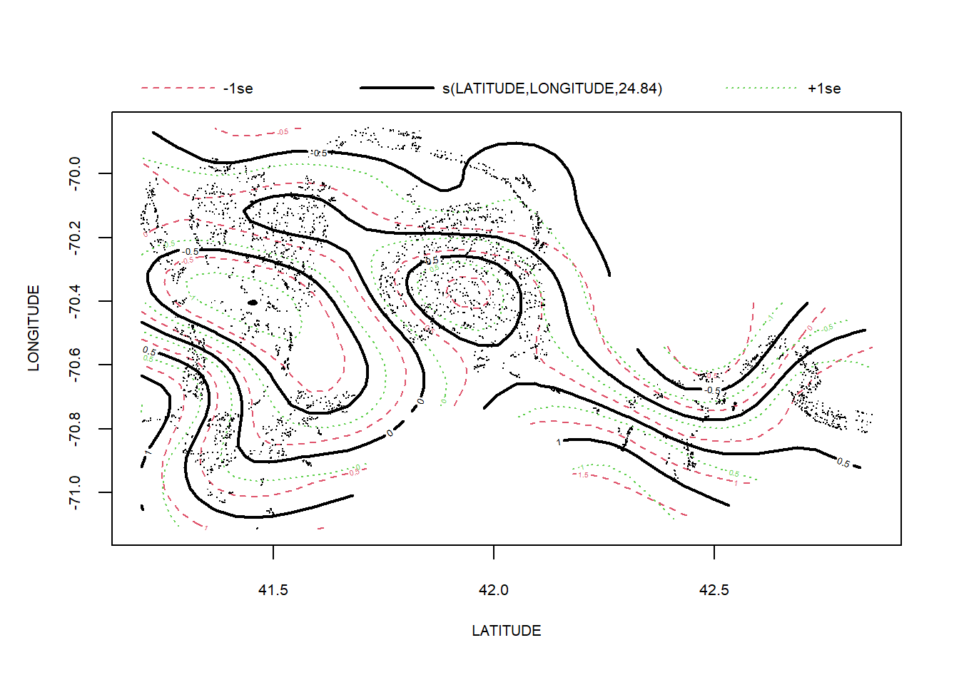
Simpson’s Evenness
#simpsons e
FV_MA_E_SP <- gamm4(E_index ~ s(FV_bot_temp) + s(FV_surf_temp) + s(FV_bot_sal) +  s(FV_surf_sal) +  s(DEPTH_M)+ s(LATITUDE, LONGITUDE) , random = ~ (1|YEAR), data = MA_spring)

gam.check(FV_MA_E_SP$gam)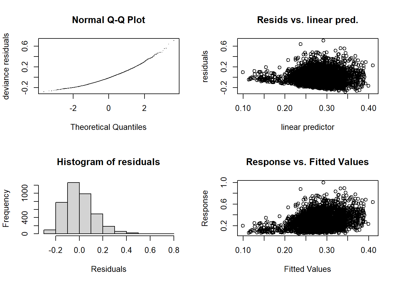
##
## 'gamm' based fit - care required with interpretation.
## Checks based on working residuals may be misleading.
## Basis dimension (k) checking results. Low p-value (k-index<1) may
## indicate that k is too low, especially if edf is close to k'.
##
##                          k'   edf k-index p-value
## s(FV_bot_temp)         9.00  2.35    1.00    0.57
## s(FV_surf_temp)        9.00  1.00    0.99    0.41
## s(FV_bot_sal)          9.00  3.44    0.99    0.36
## s(FV_surf_sal)         9.00  1.00    1.01    0.72
## s(DEPTH_M)             9.00  3.21    0.93  <2e-16 ***
## s(LATITUDE,LONGITUDE) 29.00 22.81    0.94  <2e-16 ***
## ---
## Signif. codes: 0 '***' 0.001 '**' 0.01 '*' 0.05 '.' 0.1 ' ' 1summary(FV_MA_E_SP$gam)##
## Family: gaussian
## Link function: identity
##
## Formula:
## E_index ~ s(FV_bot_temp) + s(FV_surf_temp) + s(FV_bot_sal) +
## s(FV_surf_sal) + s(DEPTH_M) + s(LATITUDE, LONGITUDE)
##
## Parametric coefficients:
## Estimate Std. Error t value Pr(>|t|)
## (Intercept) 0.280270 0.004333 64.68 <2e-16 ***
## ---
## Signif. codes: 0 '***' 0.001 '**' 0.01 '*' 0.05 '.' 0.1 ' ' 1
##
## Approximate significance of smooth terms:
## edf Ref.df F p-value
## s(FV_bot_temp) 2.349 2.349 1.009 0.3751
## s(FV_surf_temp) 1.000 1.000 0.204 0.6518
## s(FV_bot_sal) 3.435 3.435 3.059 0.0151 *
## s(FV_surf_sal) 1.000 1.000 4.506 0.0338 *
## s(DEPTH_M) 3.212 3.212 7.556 4e-05 ***
## s(LATITUDE,LONGITUDE) 22.805 22.805 7.016 <2e-16 ***
## ---
## Signif. codes: 0 '***' 0.001 '**' 0.01 '*' 0.05 '.' 0.1 ' ' 1
##
## R-sq.(adj) = 0.0946
## lmer.REML = -4960.9 Scale est. = 0.015485 n = 3877plot(FV_MA_E_SP$gam)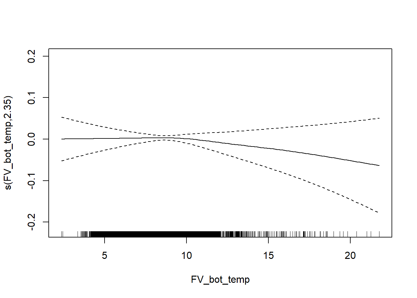
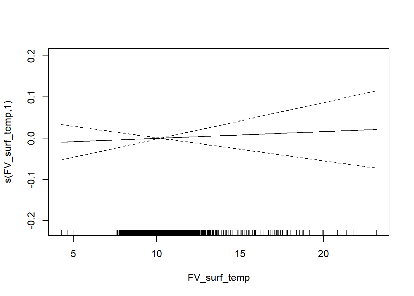
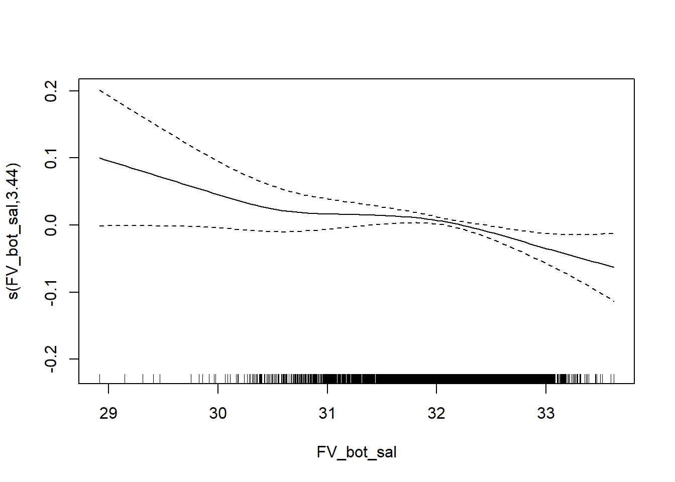
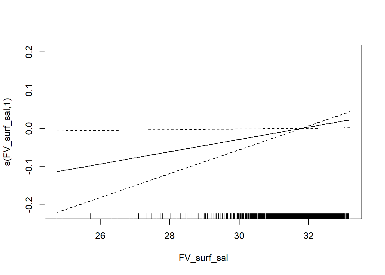
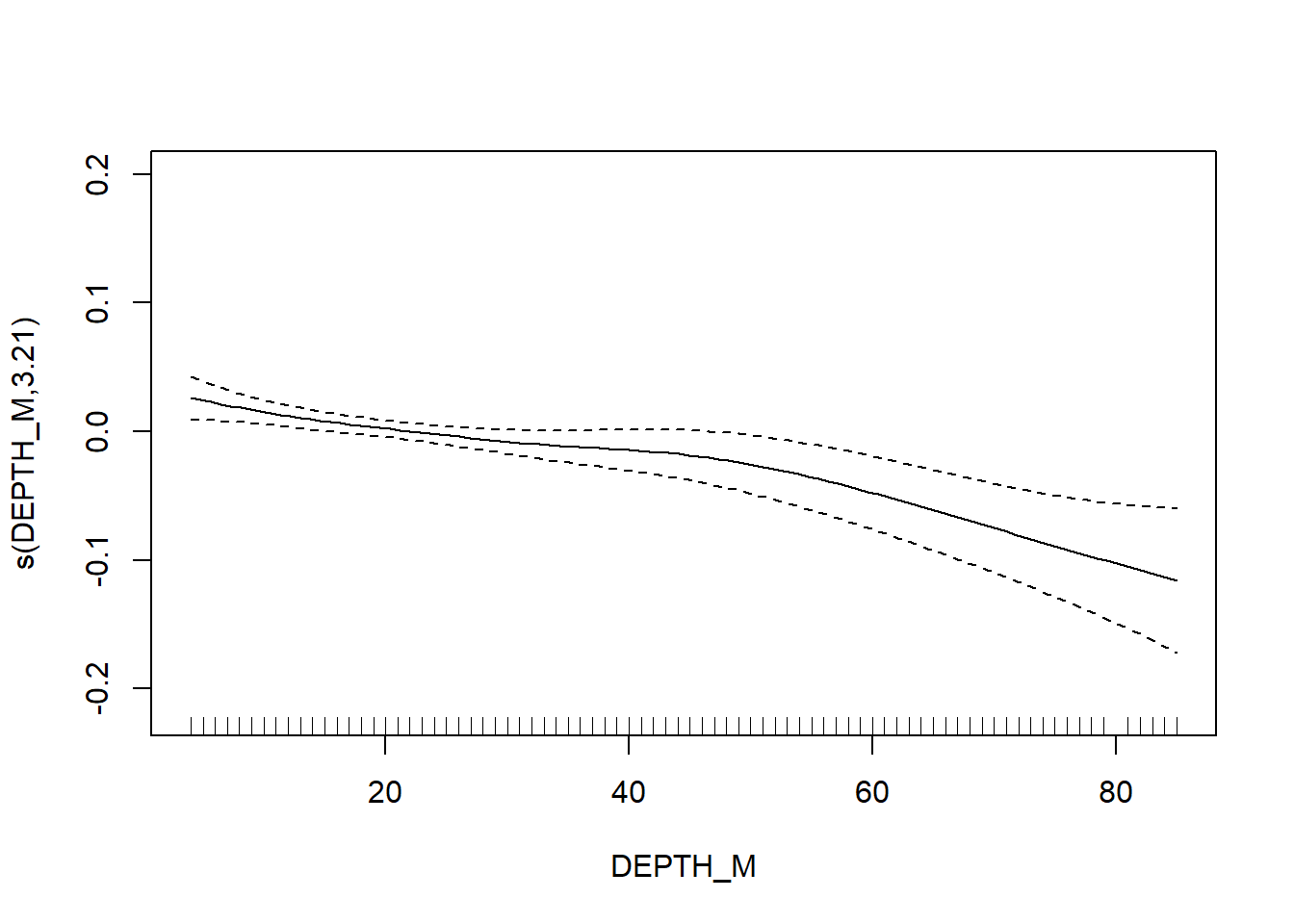
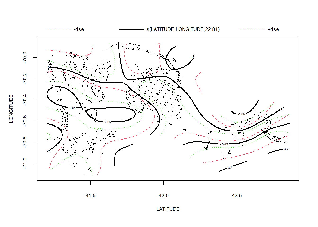
Taxonomic diversity
#tax diversity
FV_MA_delta_SP <- gamm4(delta ~ s(FV_bot_temp) + s(FV_surf_temp) + s(FV_bot_sal) +  s(FV_surf_sal) +  s(DEPTH_M)+ s(LATITUDE, LONGITUDE) , random = ~ (1|YEAR), data = MA_spring)

gam.check(FV_MA_delta_SP$gam)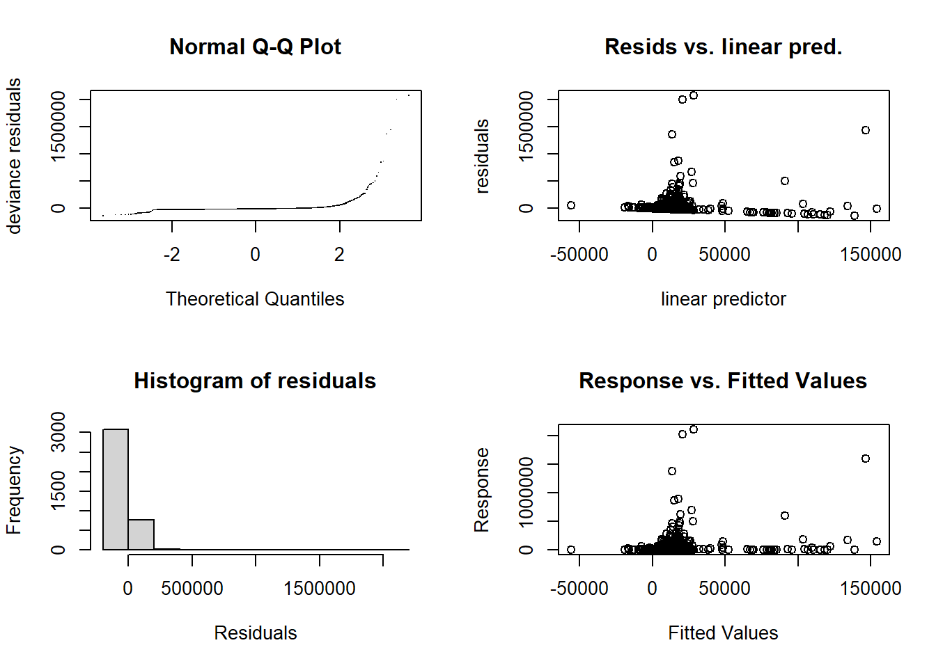
##
## 'gamm' based fit - care required with interpretation.
## Checks based on working residuals may be misleading.
## Basis dimension (k) checking results. Low p-value (k-index<1) may
## indicate that k is too low, especially if edf is close to k'.
##
##                          k'   edf k-index p-value
## s(FV_bot_temp)         9.00  4.21    1.02    0.99
## s(FV_surf_temp)        9.00  7.86    1.01    0.98
## s(FV_bot_sal)          9.00  1.00    1.01    0.96
## s(FV_surf_sal)         9.00  1.00    1.01    0.76
## s(DEPTH_M)             9.00  1.00    1.00    0.28
## s(LATITUDE,LONGITUDE) 29.00 9.98 1.04 0.66summary(FV_MA_delta_SP$gam)##
## Family: gaussian
## Link function: identity
##
## Formula:
## delta ~ s(FV_bot_temp) + s(FV_surf_temp) + s(FV_bot_sal) + s(FV_surf_sal) +
## s(DEPTH_M) + s(LATITUDE, LONGITUDE)
##
## Parametric coefficients:
## Estimate Std. Error t value Pr(>|t|)
## (Intercept) 11853 1727 6.864 7.8e-12 ***
## ---
## Signif. codes: 0 '***' 0.001 '**' 0.01 '*' 0.05 '.' 0.1 ' ' 1
##
## Approximate significance of smooth terms:
## edf Ref.df F p-value
## s(FV_bot_temp) 4.212 4.212 1.960 0.088425 .
## s(FV_surf_temp) 7.864 7.864 3.154 0.000835 ***
## s(FV_bot_sal) 1.000 1.000 0.188 0.664754
## s(FV_surf_sal) 1.000 1.000 0.195 0.658598
## s(DEPTH_M) 1.000 1.000 0.721 0.395821
## s(LATITUDE,LONGITUDE) 9.978 9.978 1.143 0.327603
## ---
## Signif. codes: 0 '***' 0.001 '**' 0.01 '*' 0.05 '.' 0.1 ' ' 1
##
## R-sq.(adj) = 0.0226
## lmer.REML = 97314 Scale est. = 4.7362e+09 n = 3877plot(FV_MA_delta_SP$gam)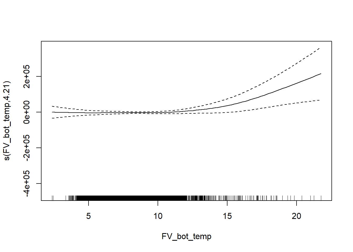
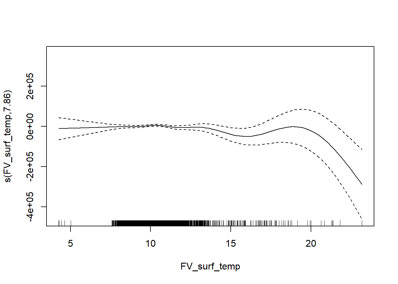
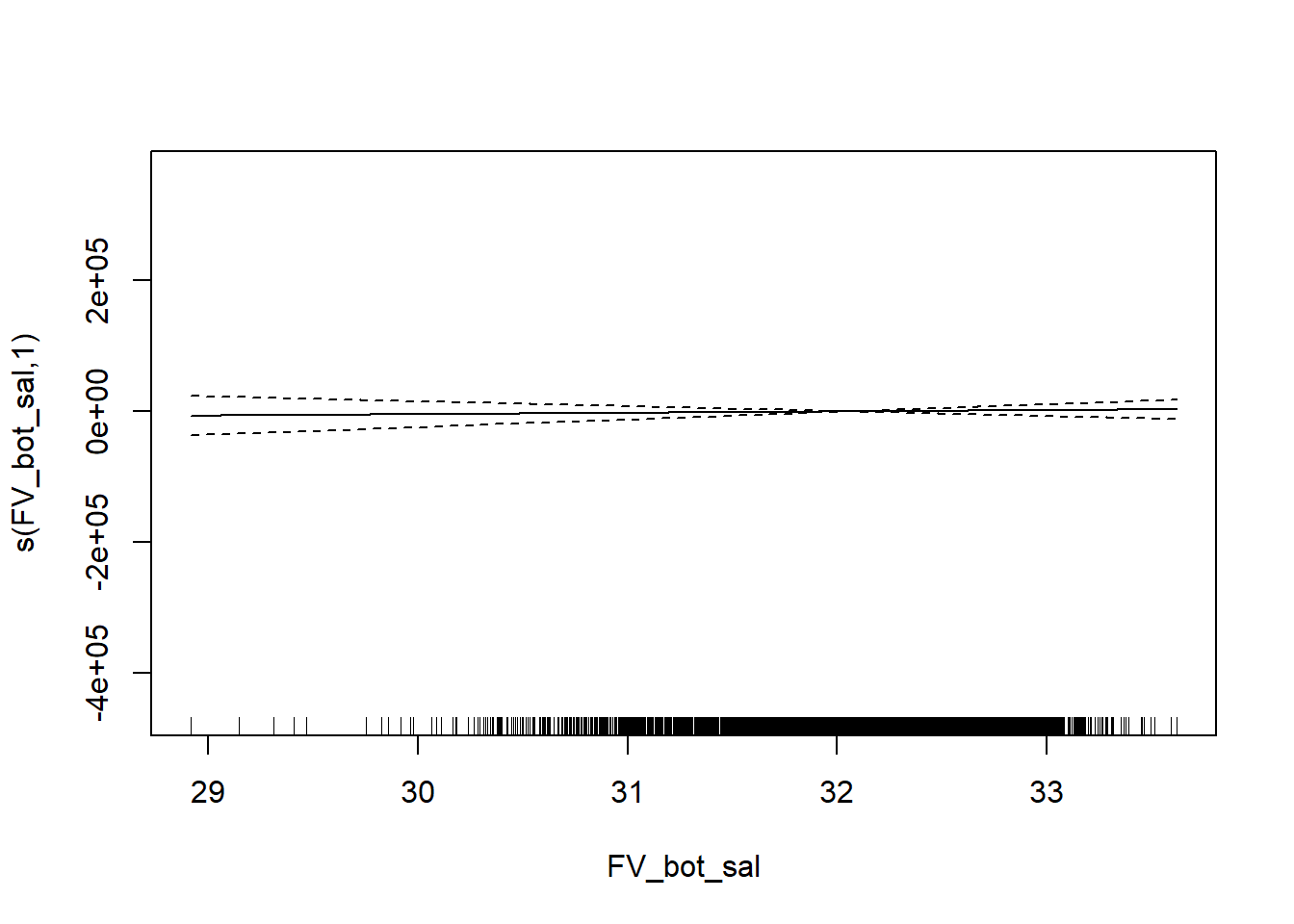
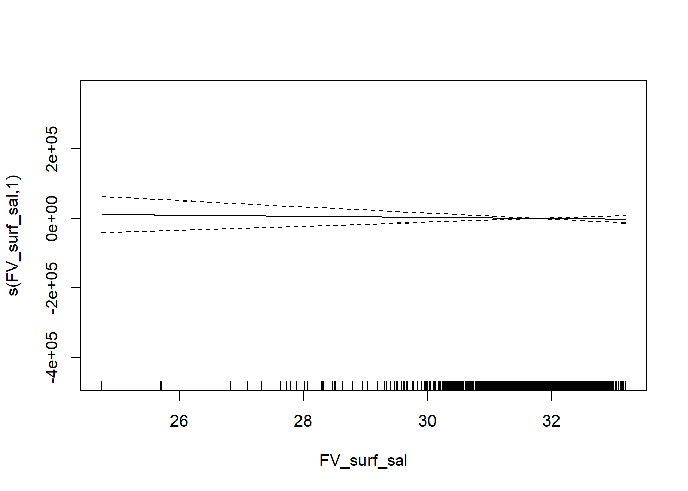
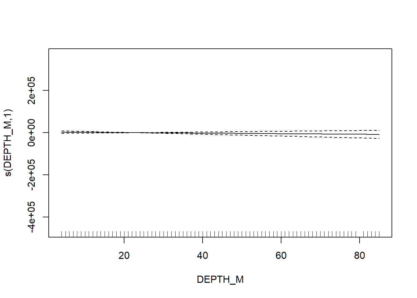
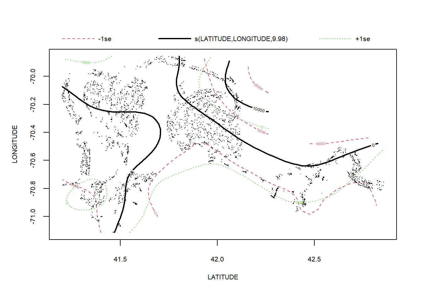
Taxonomic distinctness
# tax distinctness
FV_MA_delta_star_SP <- gamm4(delta_star ~ s(FV_bot_temp) + s(FV_surf_temp) + s(FV_bot_sal) +  s(FV_surf_sal) +  s(DEPTH_M)+ s(LATITUDE, LONGITUDE) , random = ~ (1|YEAR), data = MA_spring)

gam.check(FV_MA_delta_star_SP$gam)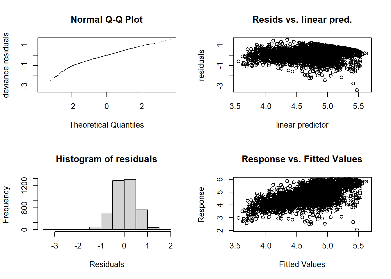
##
## 'gamm' based fit - care required with interpretation.
## Checks based on working residuals may be misleading.
## Basis dimension (k) checking results. Low p-value (k-index<1) may
## indicate that k is too low, especially if edf is close to k'.
##
##                          k'   edf k-index p-value
## s(FV_bot_temp)         9.00  5.05    1.00    0.52
## s(FV_surf_temp)        9.00  4.88    1.01    0.68
## s(FV_bot_sal)          9.00  3.62    1.00    0.41
## s(FV_surf_sal)         9.00  4.48    0.98    0.12
## s(DEPTH_M)             9.00  5.04    0.88  <2e-16 ***
## s(LATITUDE,LONGITUDE) 29.00 26.57    0.94  <2e-16 ***
## ---
## Signif. codes: 0 '***' 0.001 '**' 0.01 '*' 0.05 '.' 0.1 ' ' 1summary(FV_MA_delta_star_SP$gam)##
## Family: gaussian
## Link function: identity
##
## Formula:
## delta_star ~ s(FV_bot_temp) + s(FV_surf_temp) + s(FV_bot_sal) +
## s(FV_surf_sal) + s(DEPTH_M) + s(LATITUDE, LONGITUDE)
##
## Parametric coefficients:
## Estimate Std. Error t value Pr(>|t|)
## (Intercept) 4.65256 0.02162 215.2 <2e-16 ***
## ---
## Signif. codes: 0 '***' 0.001 '**' 0.01 '*' 0.05 '.' 0.1 ' ' 1
##
## Approximate significance of smooth terms:
## edf Ref.df F p-value
## s(FV_bot_temp) 5.046 5.046 3.081 0.008280 **
## s(FV_surf_temp) 4.881 4.881 0.807 0.541894
## s(FV_bot_sal) 3.622 3.622 3.261 0.032213 *
## s(FV_surf_sal) 4.476 4.476 4.294 0.000844 ***
## s(DEPTH_M) 5.044 5.044 10.550 < 2e-16 ***
## s(LATITUDE,LONGITUDE) 26.567 26.567 15.607 < 2e-16 ***
## ---
## Signif. codes: 0 '***' 0.001 '**' 0.01 '*' 0.05 '.' 0.1 ' ' 1
##
## R-sq.(adj) = 0.375
## lmer.REML = 5628.6 Scale est. = 0.23433 n = 3877plot(FV_MA_delta_star_SP$gam)
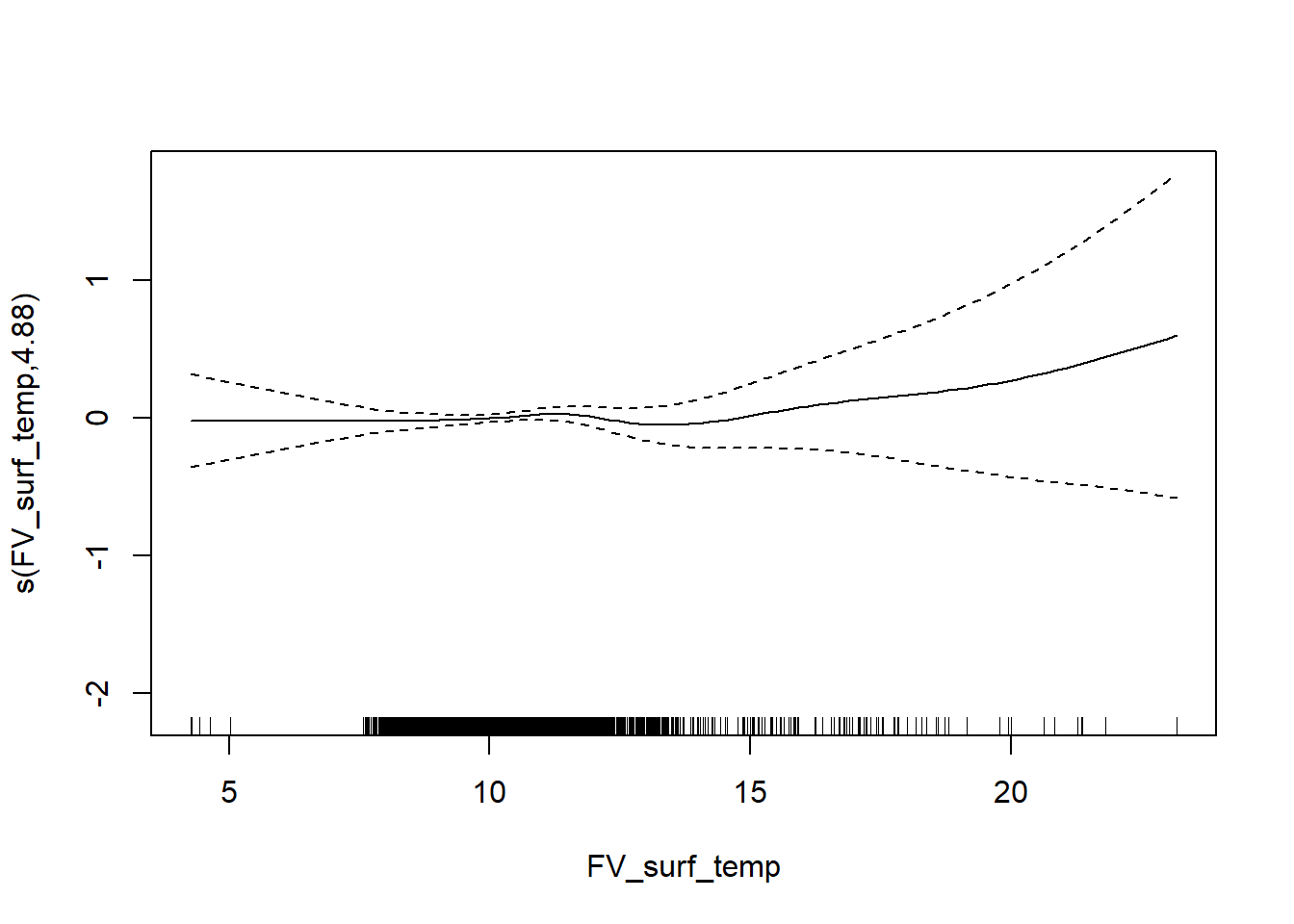
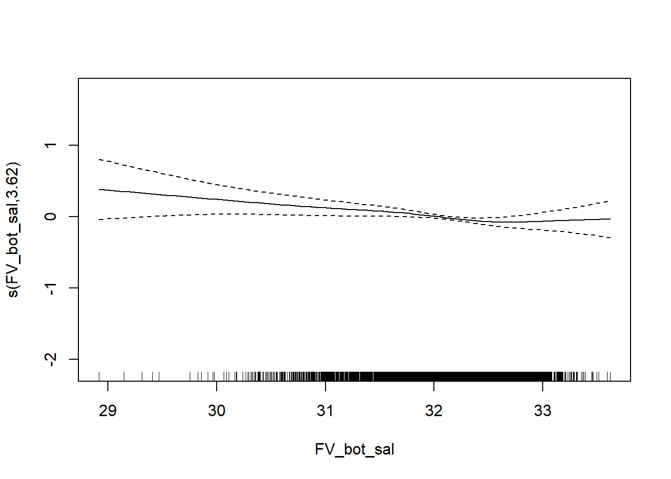
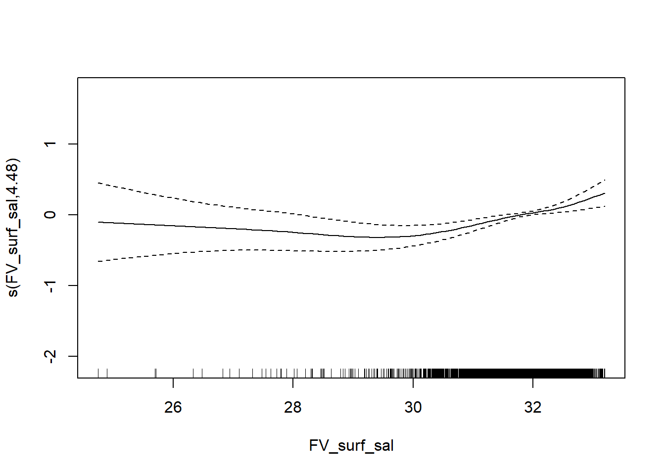
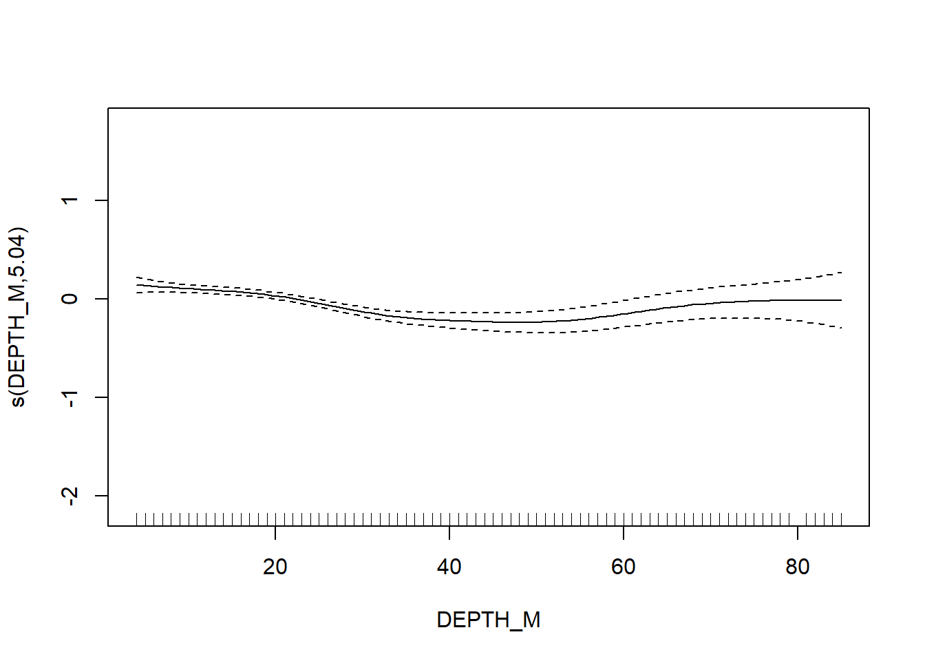
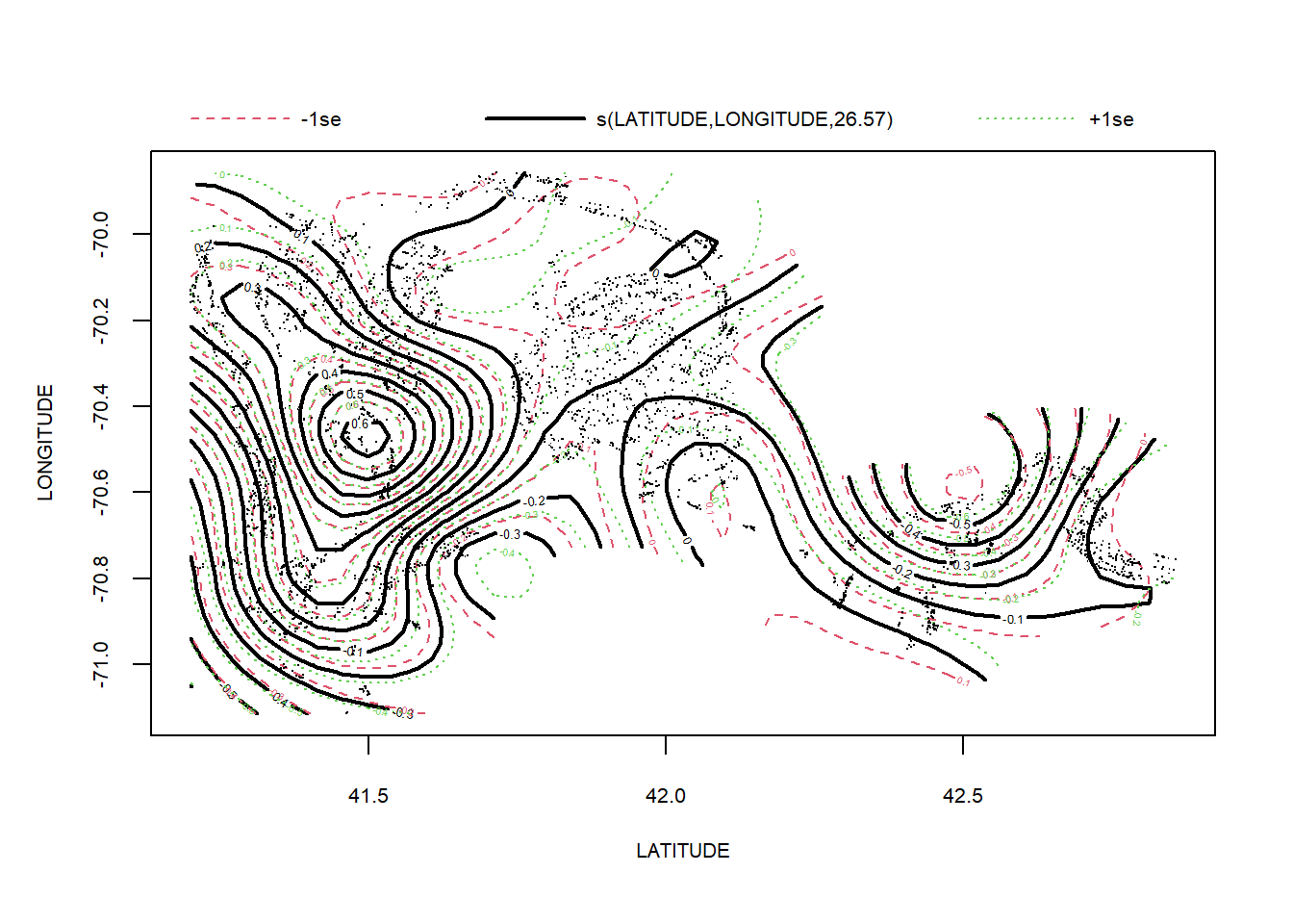
Average taxonomic distinctness
# avg tax distinctness
FV_MA_delta_plus_SP <- gamm4(delta_plus ~ s(FV_bot_temp) + s(FV_surf_temp) + s(FV_bot_sal) +  s(FV_surf_sal) + s(DEPTH_M)+ s(LATITUDE, LONGITUDE) , random = ~ (1|YEAR), data = MA_spring)

gam.check(FV_MA_delta_plus_SP$gam)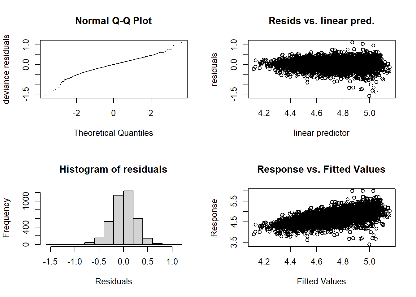
##
## 'gamm' based fit - care required with interpretation.
## Checks based on working residuals may be misleading.
## Basis dimension (k) checking results. Low p-value (k-index<1) may
## indicate that k is too low, especially if edf is close to k'.
##
##                          k'   edf k-index p-value
## s(FV_bot_temp)         9.00  4.00    0.98   0.045 *
## s(FV_surf_temp)        9.00  5.53    1.01   0.780
## s(FV_bot_sal)          9.00  4.88    0.97   0.035 *
## s(FV_surf_sal)         9.00  6.30    0.99   0.295
## s(DEPTH_M)             9.00  2.65    0.89  <2e-16 ***
## s(LATITUDE,LONGITUDE) 29.00 27.02    0.92  <2e-16 ***
## ---
## Signif. codes: 0 '***' 0.001 '**' 0.01 '*' 0.05 '.' 0.1 ' ' 1summary(FV_MA_delta_plus_SP$gam)##
## Family: gaussian
## Link function: identity
##
## Formula:
## delta_plus ~ s(FV_bot_temp) + s(FV_surf_temp) + s(FV_bot_sal) +
## s(FV_surf_sal) + s(DEPTH_M) + s(LATITUDE, LONGITUDE)
##
## Parametric coefficients:
## Estimate Std. Error t value Pr(>|t|)
## (Intercept) 4.74139 0.01175 403.6 <2e-16 ***
## ---
## Signif. codes: 0 '***' 0.001 '**' 0.01 '*' 0.05 '.' 0.1 ' ' 1
##
## Approximate significance of smooth terms:
## edf Ref.df F p-value
## s(FV_bot_temp) 4.004 4.004 4.277 0.001847 **
## s(FV_surf_temp) 5.532 5.532 4.020 0.000549 ***
## s(FV_bot_sal) 4.878 4.878 5.159 0.000132 ***
## s(FV_surf_sal) 6.300 6.300 4.834 5.12e-05 ***
## s(DEPTH_M) 2.645 2.645 18.525 < 2e-16 ***
## s(LATITUDE,LONGITUDE) 27.024 27.024 15.123 < 2e-16 ***
## ---
## Signif. codes: 0 '***' 0.001 '**' 0.01 '*' 0.05 '.' 0.1 ' ' 1
##
## R-sq.(adj) = 0.361
## lmer.REML = 256.85 Scale est. = 0.058239 n = 3877plot(FV_MA_delta_plus_SP$gam)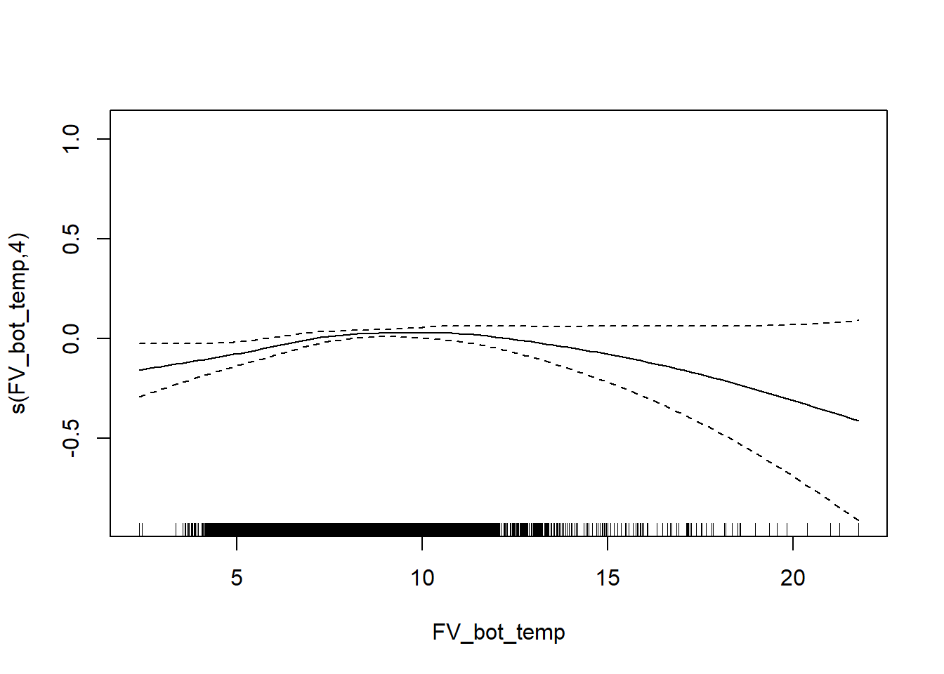
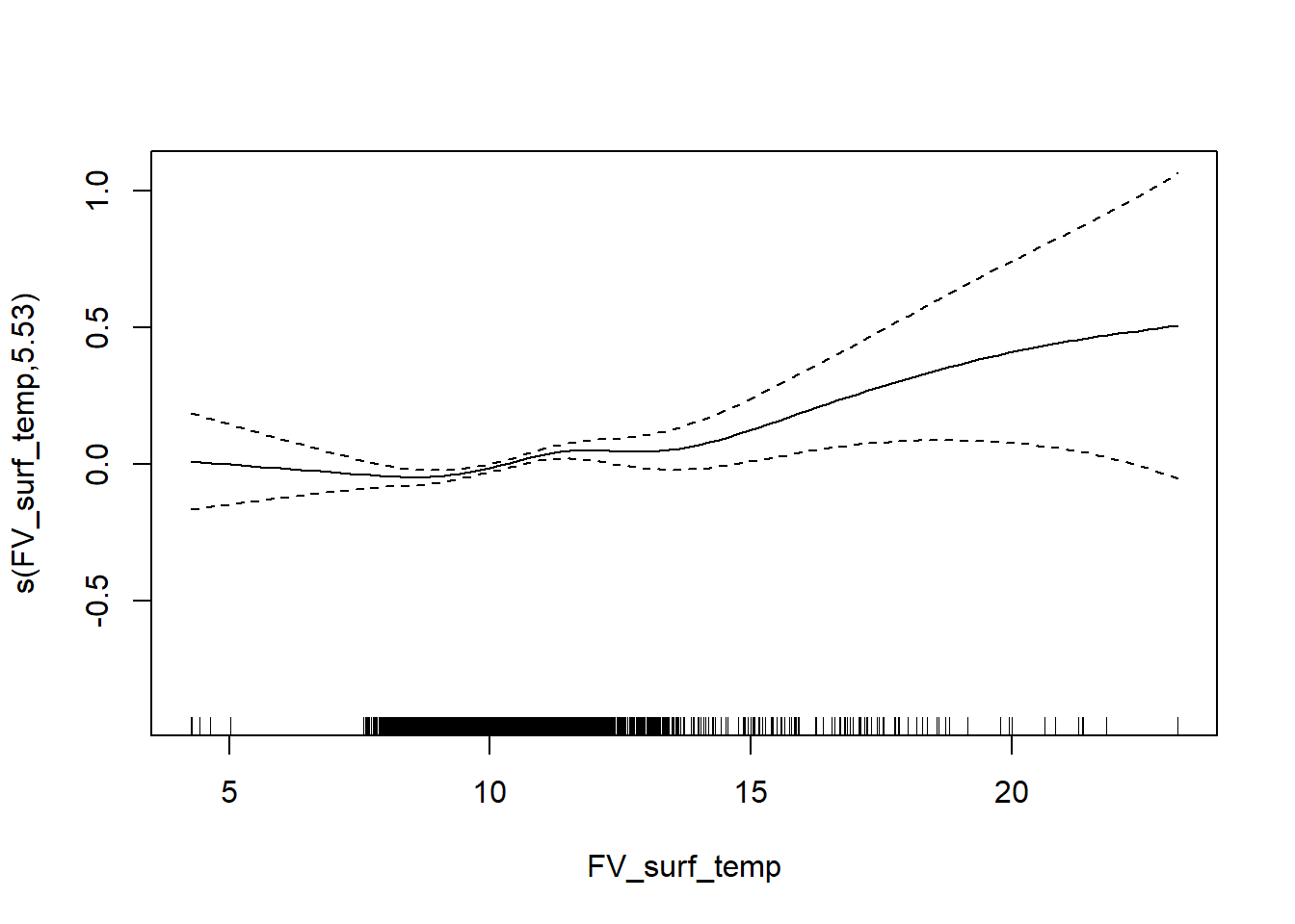
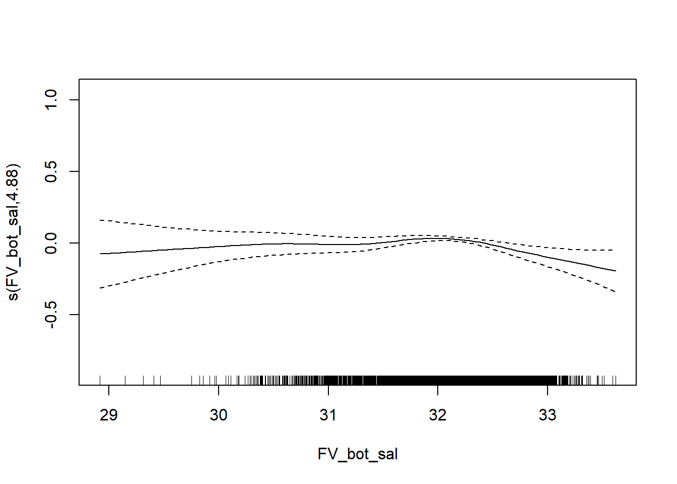
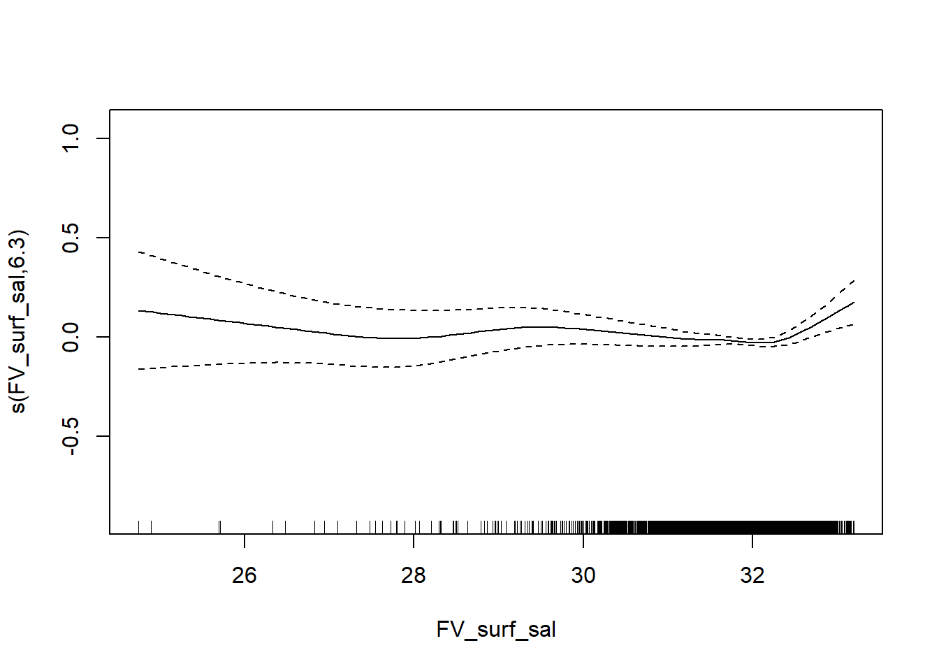
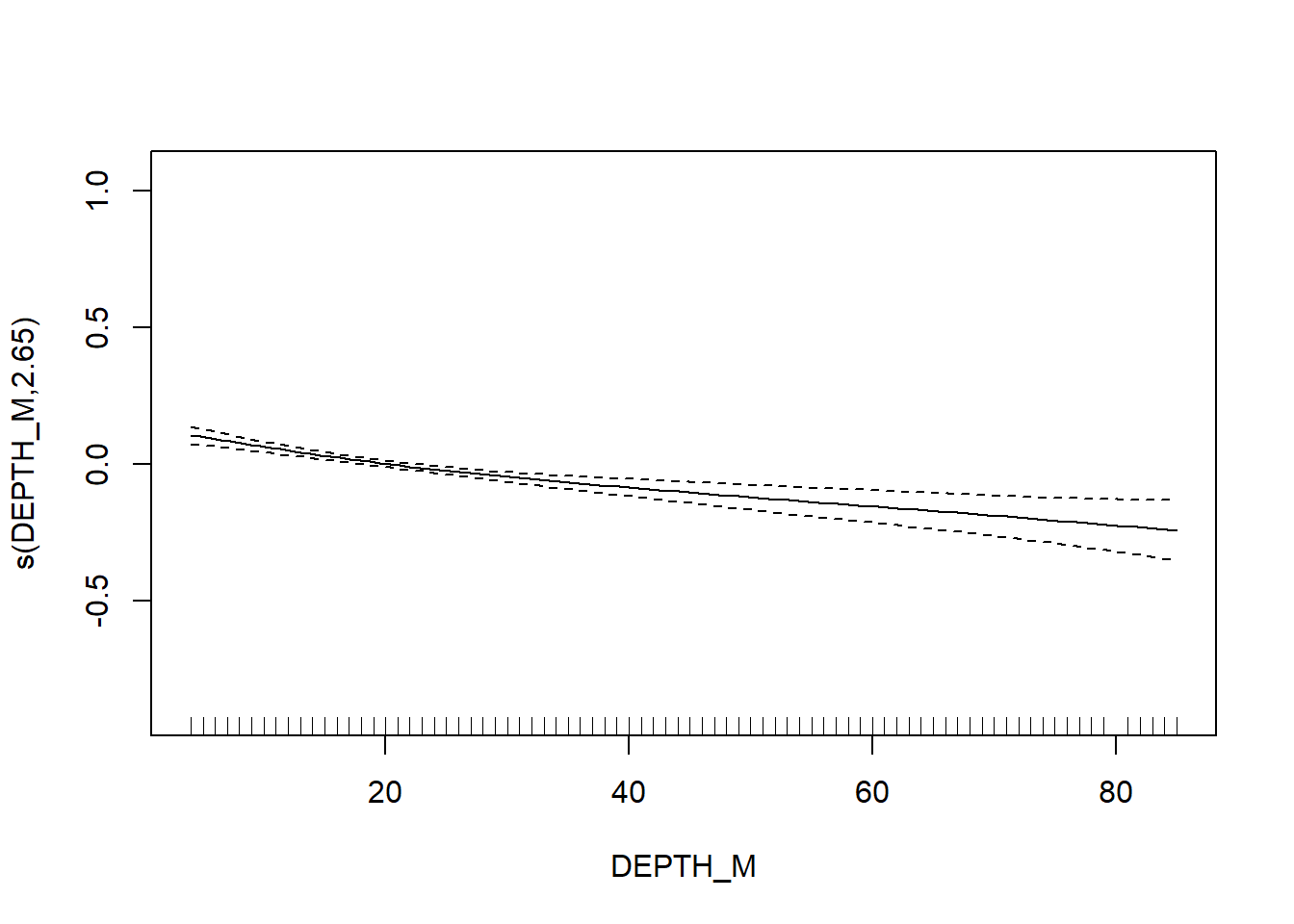
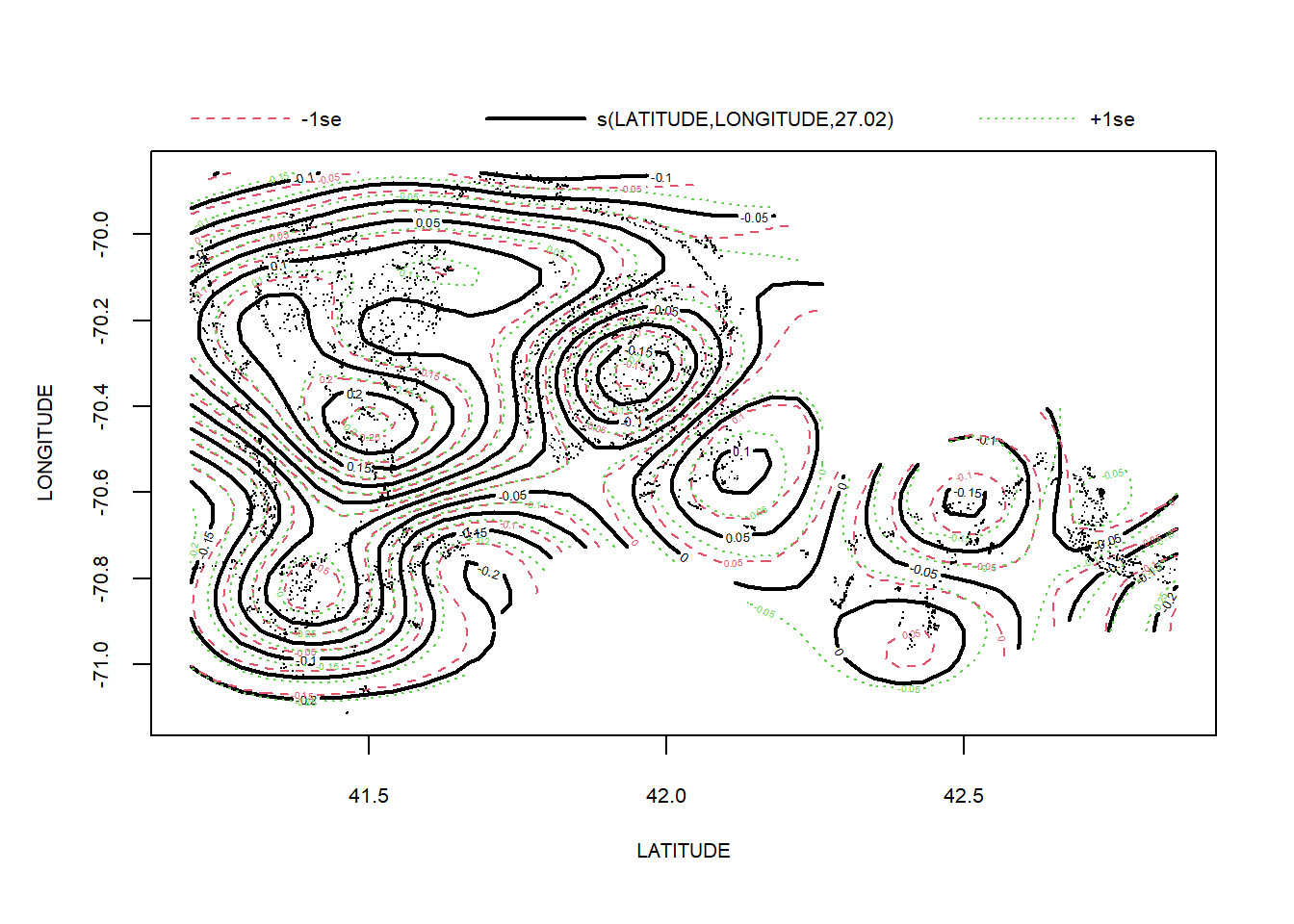
Variation in taxonomic distinctness
# var in tax distinctness
FV_MA_delta_var_SP <- gamm4(delta_var ~ s(FV_bot_temp) + s(FV_surf_temp) + s(FV_bot_sal) + s(FV_surf_sal) + s(DEPTH_M)+ s(LATITUDE, LONGITUDE) , random = ~ (1|YEAR), data = MA_spring)
gam.check(FV_MA_delta_var_SP$gam)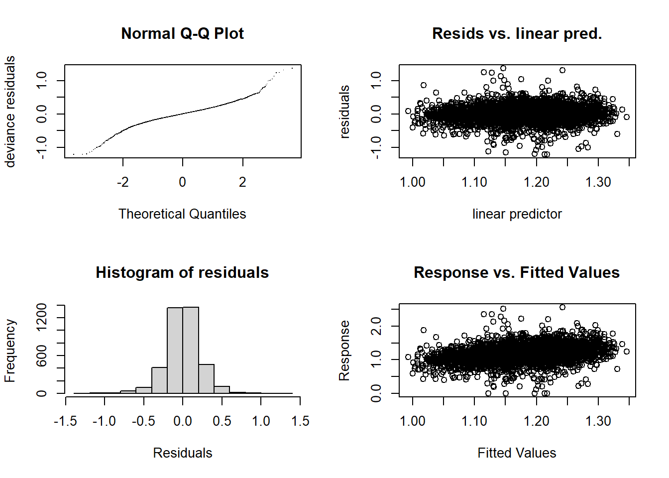
##
## 'gamm' based fit - care required with interpretation.
## Checks based on working residuals may be misleading.
## Basis dimension (k) checking results. Low p-value (k-index<1) may
## indicate that k is too low, especially if edf is close to k'.
##
## k' edf k-index p-value
## s(FV_bot_temp) 9.00 3.37 1.04 0.99
## s(FV_surf_temp) 9.00 1.00 1.00 0.34
## s(FV_bot_sal) 9.00 2.53 0.97 0.06 .
## s(FV_surf_sal) 9.00 1.00 0.99 0.25
## s(DEPTH_M) 9.00 3.66 0.95 <2e-16 ***
## s(LATITUDE,LONGITUDE) 29.00 23.28 0.95 <2e-16 ***
## ---
## Signif. codes: 0 '***' 0.001 '**' 0.01 '*' 0.05 '.' 0.1 ' ' 1summary(FV_MA_delta_var_SP$gam)##
## Family: gaussian
## Link function: identity
##
## Formula:
## delta_var ~ s(FV_bot_temp) + s(FV_surf_temp) + s(FV_bot_sal) +
## s(FV_surf_sal) + s(DEPTH_M) + s(LATITUDE, LONGITUDE)
##
## Parametric coefficients:
## Estimate Std. Error t value Pr(>|t|)
## (Intercept) 1.181246 0.007778 151.9 <2e-16 ***
## ---
## Signif. codes: 0 '***' 0.001 '**' 0.01 '*' 0.05 '.' 0.1 ' ' 1
##
## Approximate significance of smooth terms:
## edf Ref.df F p-value
## s(FV_bot_temp) 3.371 3.371 1.945 0.19760
## s(FV_surf_temp) 1.000 1.000 1.271 0.25959
## s(FV_bot_sal) 2.535 2.535 3.266 0.02213 *
## s(FV_surf_sal) 1.000 1.000 0.850 0.35652
## s(DEPTH_M) 3.660 3.660 4.088 0.00351 **
## s(LATITUDE,LONGITUDE) 23.276 23.276 7.305 < 2e-16 ***
## ---
## Signif. codes: 0 '***' 0.001 '**' 0.01 '*' 0.05 '.' 0.1 ' ' 1
##
## R-sq.(adj) = 0.0807
## lmer.REML = -269.57 Scale est. = 0.052028 n = 3877plot(FV_MA_delta_var_SP$gam)