Environmental Effects on Community structure NMDS
includes latitude, longitude, salinity, temperature, depth
Functional Group Biomass
NMDS
#load in data
trawl_data_arrange<-read.csv(here("Data/group_biomass_matrix.csv"))[-1]

trawl_data<-read.csv(here("Data/MaineDMR_Trawl_Survey_Tow_Data_2021-05-14.csv"))

all_Data<-group_by(trawl_data, Season, Year, Region)%>%
  filter(Year<2020)%>%
  summarise(start_lat=mean(Start_Latitude),start_long=mean(Start_Longitude),end_lat=mean(End_Latitude), end_long=mean(End_Longitude),start_depth=mean(Start_Depth_fathoms, na.rm=TRUE), end_depth=mean(End_Depth_fathoms, na.rm=TRUE), bottom_temp=mean(Bottom_WaterTemp_DegC, na.rm=TRUE), bottom_sal=mean(Bottom_Salinity, na.rm=TRUE),surface_temp=mean(Surface_WaterTemp_DegC, na.rm=TRUE), surface_sal=mean(Surface_Salinity, na.rm=TRUE))%>%
  full_join(trawl_data_arrange)%>%
  ungroup()

com<-select(all_Data, benthivore, benthos,piscivore,planktivore, undefined)

com<-vegdist(com, method="bray")

#convert com to a matrix
m_com = as.matrix(com)

set.seed(123)
nmds = metaMDS(m_com,k=2, distance = "bray", trymax = 200)
## Run 0 stress 0.1741426
## Run 1 stress 0.1741425
## ... New best solution
## ... Procrustes: rmse 8.547141e-05 max resid 0.001121714
## ... Similar to previous best
## Run 2 stress 0.1741403
## ... New best solution
## ... Procrustes: rmse 0.0006325414 max resid 0.008146205
## ... Similar to previous best
## Run 3 stress 0.1741405
## ... Procrustes: rmse 7.796045e-05 max resid 0.0009075655
## ... Similar to previous best
## Run 4 stress 0.174143
## ... Procrustes: rmse 0.000617407 max resid 0.007835139
## ... Similar to previous best
## Run 5 stress 0.1756323
## Run 6 stress 0.1741425
## ... Procrustes: rmse 0.0006070086 max resid 0.007888487
## ... Similar to previous best
## Run 7 stress 0.1741427
## ... Procrustes: rmse 0.0006227408 max resid 0.007964962
## ... Similar to previous best
## Run 8 stress 0.1773435
## Run 9 stress 0.1774551
## Run 10 stress 0.1868927
## Run 11 stress 0.1833826
## Run 12 stress 0.1756293
## Run 13 stress 0.1792026
## Run 14 stress 0.1873262
## Run 15 stress 0.1792051
## Run 16 stress 0.1873265
## Run 17 stress 0.1741427
## ... Procrustes: rmse 0.0006111671 max resid 0.007892951
## ... Similar to previous best
## Run 18 stress 0.175632
## Run 19 stress 0.1792018
## Run 20 stress 0.1741426
## ... Procrustes: rmse 0.0006109017 max resid 0.007909025
## ... Similar to previous best
## *** Solution reachednmds##
## Call:
## metaMDS(comm = m_com, distance = "bray", k = 2, trymax = 200)
##
## global Multidimensional Scaling using monoMDS
##
## Data: m_com
## Distance: user supplied
##
## Dimensions: 2
## Stress: 0.1741403
## Stress type 1, weak ties
## Two convergent solutions found after 20 tries
## Scaling: centring, PC rotation
## Species: scores missingEnvfit
env<-select(all_Data, start_lat, start_long, end_lat, end_long,start_depth, end_depth, bottom_temp, bottom_sal, surface_temp, surface_sal)

en<-envfit(nmds, env, permutations=999, na.rm=TRUE)
en
##
## ***VECTORS
##
## NMDS1 NMDS2 r2 Pr(>r)
## start_lat 0.38259 -0.92392 0.1461 0.001 ***
## start_long 0.29706 -0.95486 0.1659 0.001 ***
## end_lat 0.37975 -0.92509 0.1454 0.001 ***
## end_long 0.29696 -0.95489 0.1659 0.001 ***
## start_depth -0.84780 -0.53031 0.0347 0.028 *
## end_depth -0.74052 -0.67203 0.0300 0.058 .
## bottom_temp -0.98891 -0.14850 0.3638 0.001 ***
## bottom_sal -0.99645 -0.08424 0.1995 0.001 ***
## surface_temp -0.96907 0.24679 0.4962 0.001 ***
## surface_sal 0.61131 0.79139 0.0008 0.927
## ---
## Signif. codes: 0 '***' 0.001 '**' 0.01 '*' 0.05 '.' 0.1 ' ' 1
## Permutation: free
## Number of permutations: 999
##
## 5 observations deleted due to missingnessplot(nmds)
plot(en)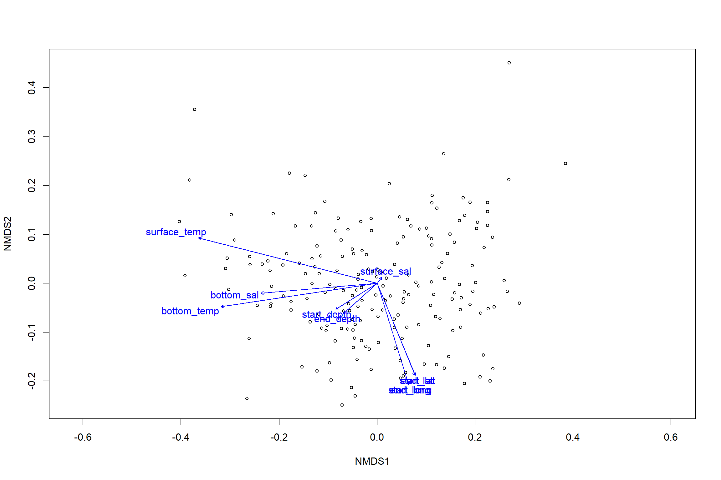
en_coord_cont = as.data.frame(scores(en, "vectors")) * ordiArrowMul(en)
en_coord_cat = as.data.frame(scores(en, "factors")) * ordiArrowMul(en)

#extract NMDS scores for ggplot
data.scores = as.data.frame(scores(nmds))
#add columns to data frame
data.scores$Region = all_Data$Region
data.scores$Year = all_Data$Year
data.scores$Season= all_Data$Season
data.scores$Year_groups= all_Data$YEAR_GROUPS
data.scores$Year_decades= all_Data$YEAR_DECADES
data.scores$Region_new=all_Data$REGION_NEW
data.scores$Region_year=all_Data$REGION_YEAR
data.scores$Season_year=all_Data$SEASON_YEAR

p<- ggplot()+
     geom_point(data = data.scores, aes(x = NMDS1, y = NMDS2, color=Year_groups, shape=Region_new), size = 4) +
  scale_color_colorblind()+
        geom_segment(data=en_coord_cont, aes(x = 0, y = 0, xend = NMDS1, yend = NMDS2), size =1.5, alpha = 0.5)+
   geom_text(data = en_coord_cont, aes(x = NMDS1, y = NMDS2), size=5,
       fontface = "bold", label = row.names(en_coord_cont))+
    theme(axis.title = element_text(size = 16, face = "bold"),
       panel.background = element_blank(), panel.border = element_rect(fill = NA),
       axis.ticks = element_blank(), axis.text = element_blank(), legend.key = element_blank(),
       legend.title = element_text(size = 16, face = "bold"),
       legend.text = element_text(size = 16))


p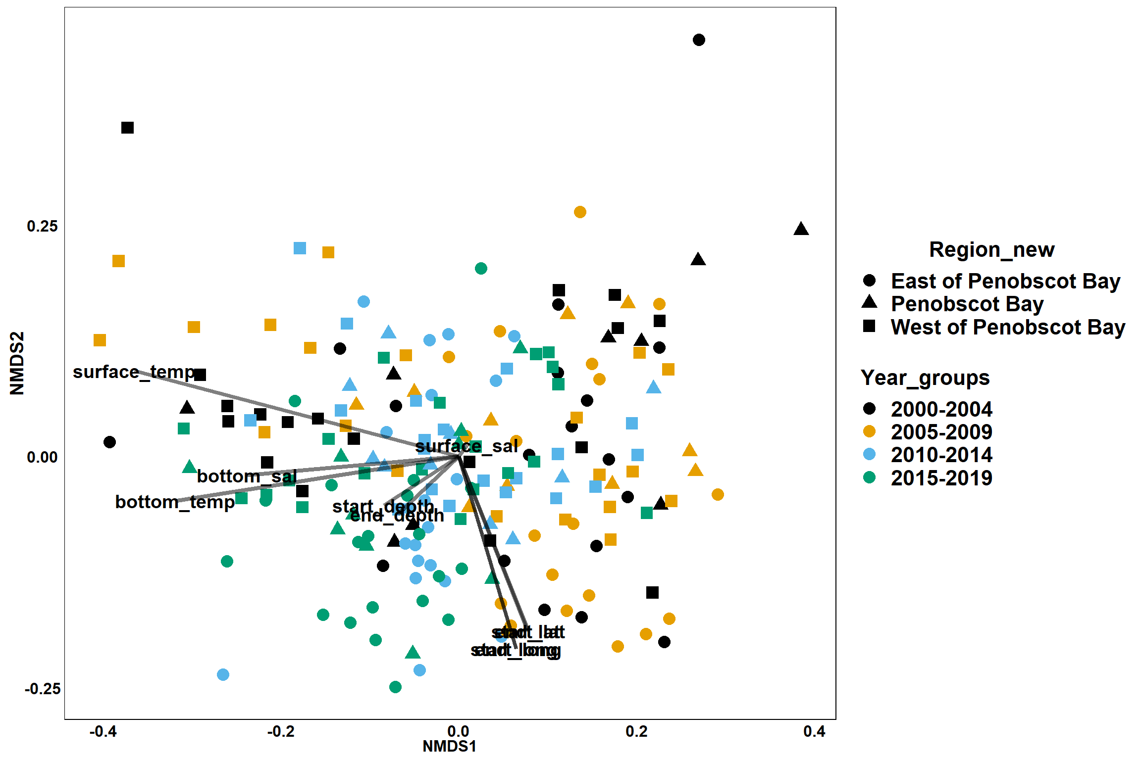
Region groups
p_region<- ggplot()+
     geom_point(data = data.scores, aes(x = NMDS1, y = NMDS2, color=Region_new), size = 4) +
  scale_color_colorblind()+
        geom_segment(data=en_coord_cont, aes(x = 0, y = 0, xend = NMDS1, yend = NMDS2), size =1.5, alpha = 0.5)+
   geom_text(data = en_coord_cont, aes(x = NMDS1, y = NMDS2), size=5,
       fontface = "bold", label = row.names(en_coord_cont))+
  stat_ellipse(data=data.scores, aes(x=NMDS1, y=NMDS2, color=Region_new),level = 0.95,size=1)+
  theme(axis.title = element_text(size = 16, face = "bold"),
       panel.background = element_blank(), panel.border = element_rect(fill = NA),
       axis.ticks = element_blank(), axis.text = element_blank(), legend.key = element_blank(),
       legend.title = element_text(size = 16, face = "bold"),
       legend.text = element_text(size = 16))


p_region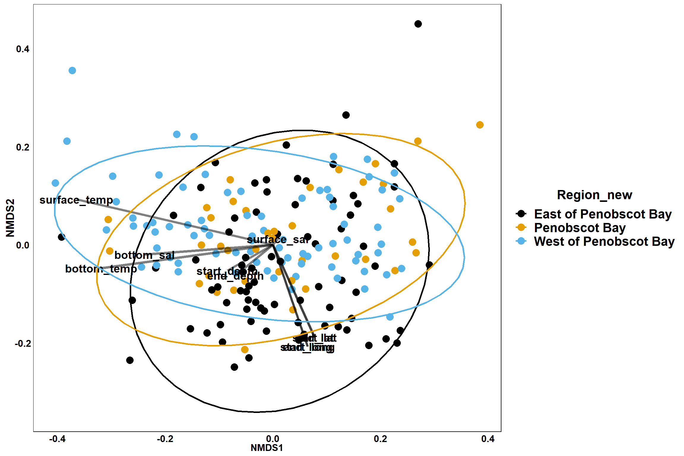
Year groups
p_year<- ggplot()+
     geom_point(data = data.scores, aes(x = NMDS1, y = NMDS2, color=Year_groups), size = 4) +
  scale_color_colorblind()+
        geom_segment(data=en_coord_cont, aes(x = 0, y = 0, xend = NMDS1, yend = NMDS2), size =1.5, alpha = 0.5)+
   geom_text(data = en_coord_cont, aes(x = NMDS1, y = NMDS2), size=5,
       fontface = "bold", label = row.names(en_coord_cont))+
  stat_ellipse(data=data.scores, aes(x=NMDS1, y=NMDS2, color=Year_groups),level = 0.95,size=1)+
  theme(axis.title = element_text(size = 16, face = "bold"),
       panel.background = element_blank(), panel.border = element_rect(fill = NA),
       axis.ticks = element_blank(), axis.text = element_blank(), legend.key = element_blank(),
       legend.title = element_text(size = 16, face = "bold"),
       legend.text = element_text(size = 16))

p_year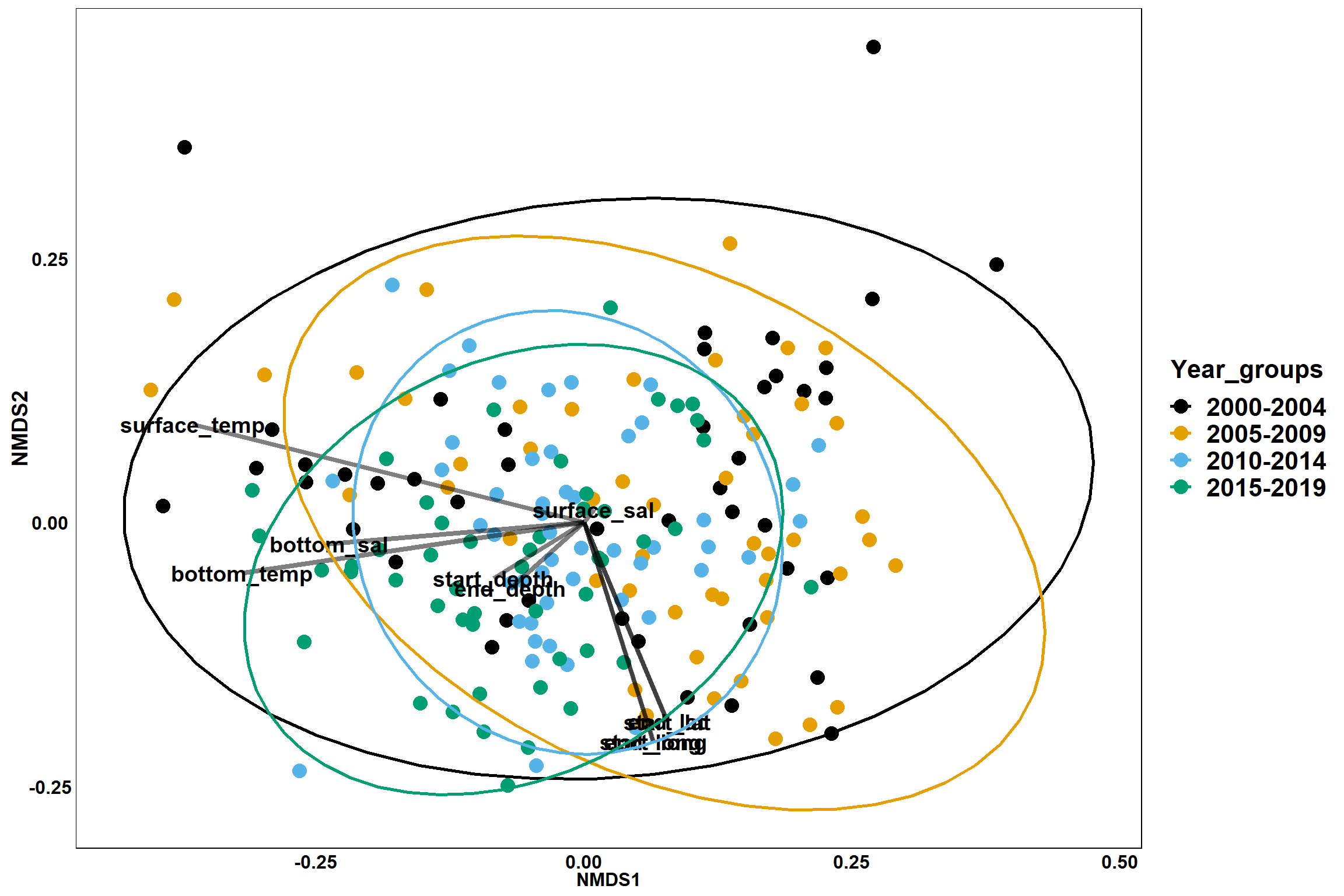
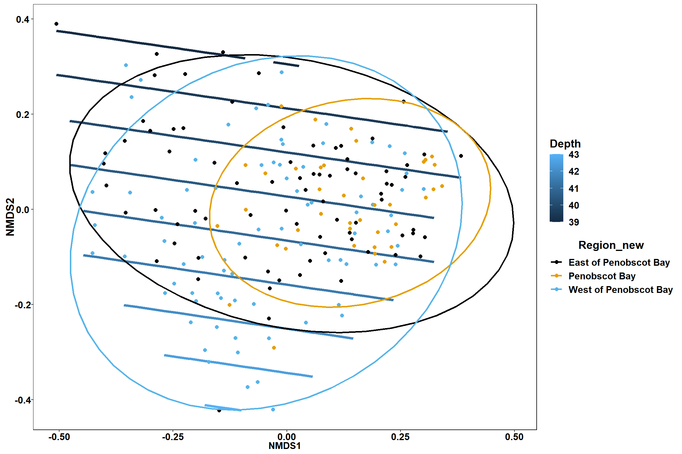
GAM contours for environmental effects
Bottom temperature
bottom_temp<-ordisurf(nmds, env$bottom_temp)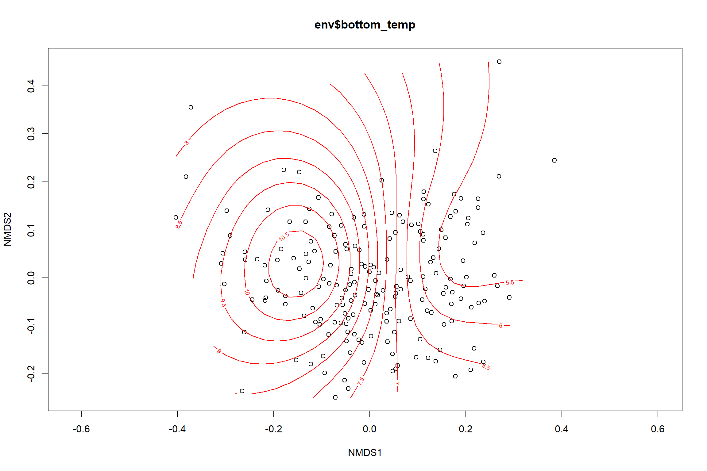
summary(bottom_temp)##
## Family: gaussian
## Link function: identity
##
## Formula:
## y ~ s(x1, x2, k = 10, bs = "tp", fx = FALSE)
##
## Parametric coefficients:
## Estimate Std. Error t value Pr(>|t|)
## (Intercept) 7.9053 0.1355 58.34 <2e-16 ***
## ---
## Signif. codes: 0 '***' 0.001 '**' 0.01 '*' 0.05 '.' 0.1 ' ' 1
##
## Approximate significance of smooth terms:
## edf Ref.df F p-value
## s(x1,x2) 6.605 9 19.65 <2e-16 ***
## ---
## Signif. codes: 0 '***' 0.001 '**' 0.01 '*' 0.05 '.' 0.1 ' ' 1
##
## R-sq.(adj) = 0.483 Deviance explained = 50.1%
## -REML = 397.4 Scale est. = 3.4884 n = 190ordi.grid <- bottom_temp$grid #extracts the ordisurf object
#str(ordi.grid) #it's a list though - cannot be plotted as is
ordi.mite <- expand.grid(x = ordi.grid$x, y = ordi.grid$y) #get x and ys
ordi.mite$z <- as.vector(ordi.grid$z) #unravel the matrix for the z scores
contour.vals <- data.frame(na.omit(ordi.mite)) #gets rid of the nas
p <- ggplot()+
stat_contour(data = contour.vals, aes(x, y, z=z, color = ..level..),position="identity",size=1.5)+
labs(x = "NMDS1", y = "NMDS2", color="Bottom Temperature")+
new_scale_color()+
geom_point(data = data.scores, aes(NMDS1, NMDS2, color=Year_groups, shape=Region_new), size = 3 )+ scale_color_colorblind()
p1 <- ggplot()+
stat_contour(data = contour.vals, aes(x, y, z=z, color = ..level..),position="identity",size=1.5)+
labs(x = "NMDS1", y = "NMDS2", color="Bottom Temperature")+
new_scale_color()+
geom_point(data = data.scores, aes(NMDS1, NMDS2, color=Year_groups), size = 2 )+ stat_ellipse(data=data.scores, aes(x=NMDS1, y=NMDS2, color=Year_groups),level = 0.95,size=1)+
scale_color_colorblind()
p2 <- ggplot()+
stat_contour(data = contour.vals, aes(x, y, z=z, color = ..level..),position="identity",size=1.5)+
labs(x = "NMDS1", y = "NMDS2", color="Bottom Temperature")+
new_scale_color()+
geom_point(data = data.scores, aes(NMDS1, NMDS2, color=Region_new), size = 2 )+
stat_ellipse(data=data.scores, aes(x=NMDS1, y=NMDS2, color=Region_new),level = 0.95,size=1)+
scale_color_colorblind()
p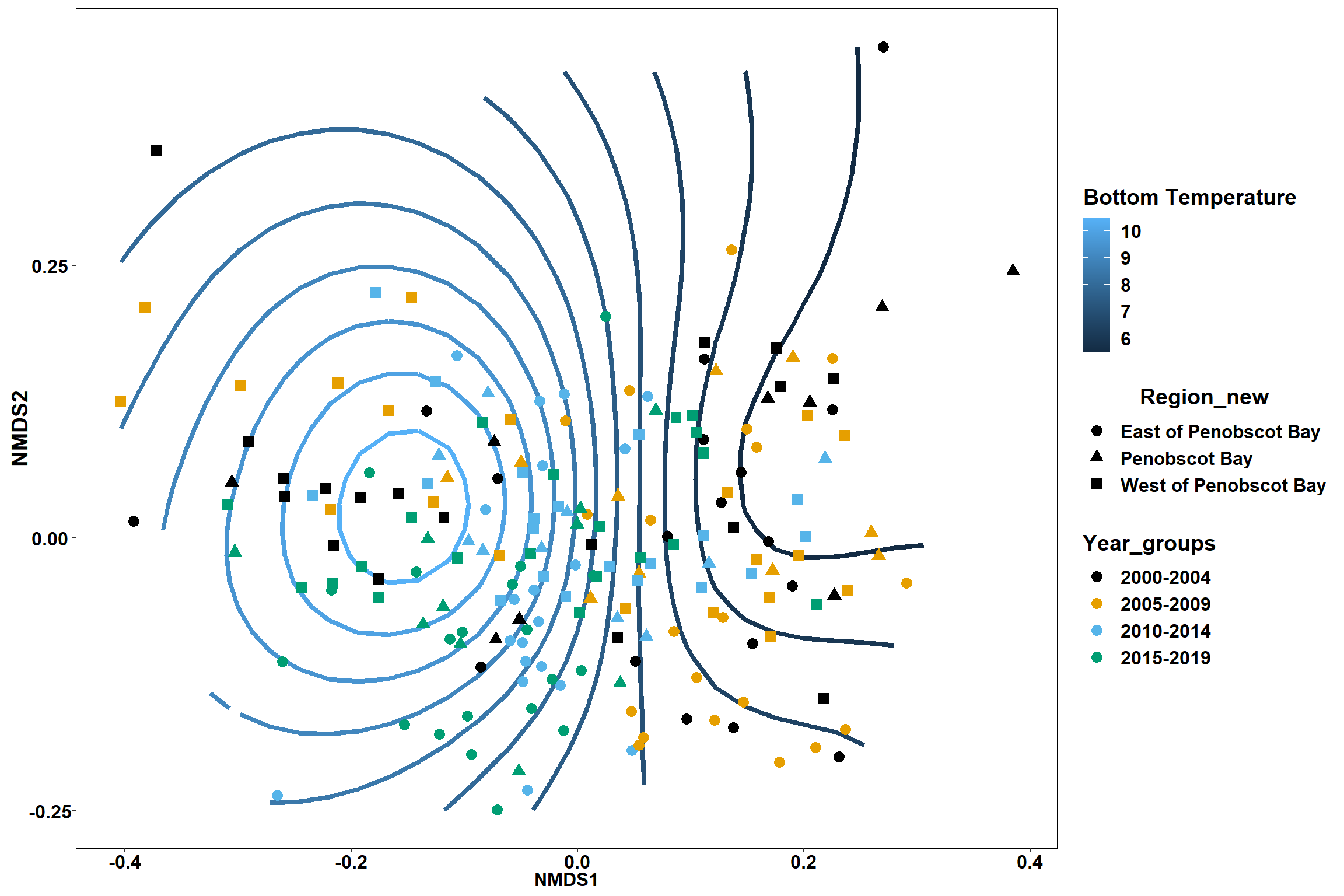
p1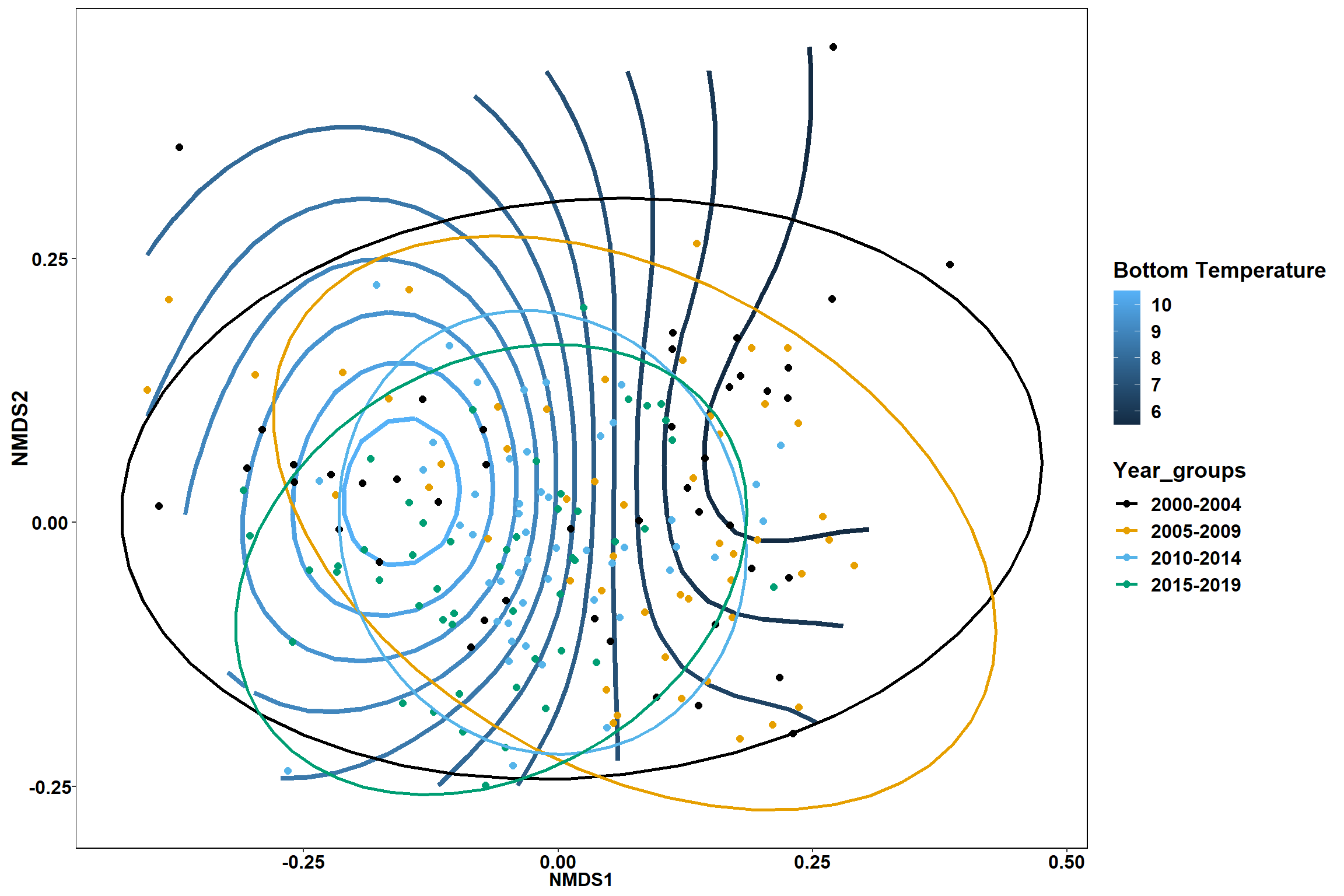
p2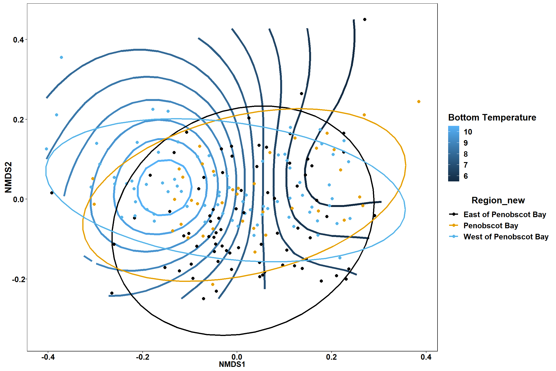
Surface temperature
surface_temp<-ordisurf(nmds, env$surface_temp)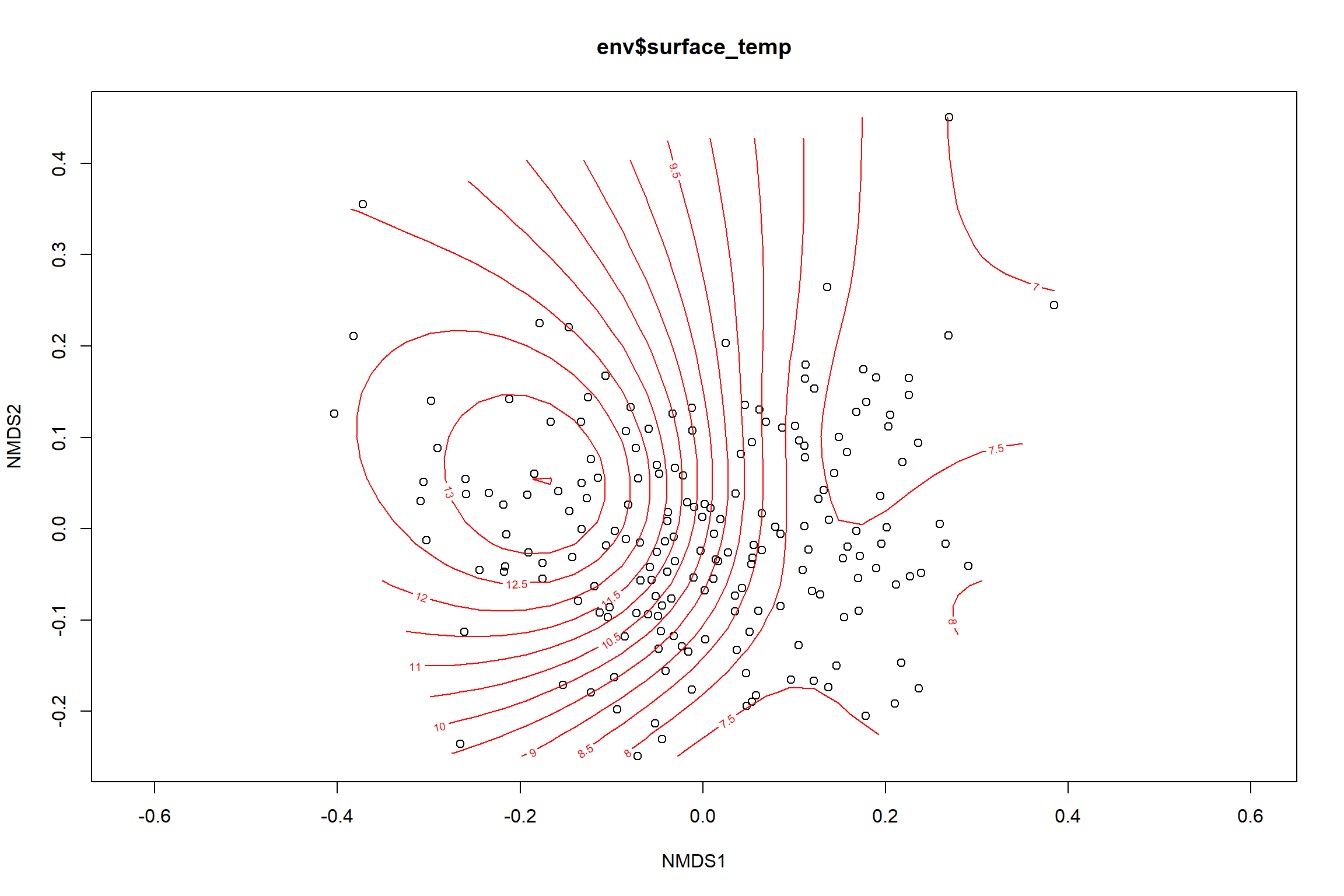
summary(surface_temp)##
## Family: gaussian
## Link function: identity
##
## Formula:
## y ~ s(x1, x2, k = 10, bs = "tp", fx = FALSE)
##
## Parametric coefficients:
## Estimate Std. Error t value Pr(>|t|)
## (Intercept) 9.7700 0.1225 79.73 <2e-16 ***
## ---
## Signif. codes: 0 '***' 0.001 '**' 0.01 '*' 0.05 '.' 0.1 ' ' 1
##
## Approximate significance of smooth terms:
## edf Ref.df F p-value
## s(x1,x2) 7.611 9 33.59 <2e-16 ***
## ---
## Signif. codes: 0 '***' 0.001 '**' 0.01 '*' 0.05 '.' 0.1 ' ' 1
##
## R-sq.(adj) = 0.615 Deviance explained = 63.1%
## -REML = 380.68 Scale est. = 2.8531 n = 190ordi.grid <- surface_temp$grid #extracts the ordisurf object
#str(ordi.grid) #it's a list though - cannot be plotted as is
ordi.mite <- expand.grid(x = ordi.grid$x, y = ordi.grid$y) #get x and ys
ordi.mite$z <- as.vector(ordi.grid$z) #unravel the matrix for the z scores
contour.vals <- data.frame(na.omit(ordi.mite)) #gets rid of the nas
p <- ggplot()+
stat_contour(data = contour.vals, aes(x, y, z=z, color = ..level..),position="identity",size=1.5)+
labs(x = "NMDS1", y = "NMDS2", color="Surface Temperature")+
new_scale_color()+
geom_point(data = data.scores, aes(NMDS1, NMDS2, color=Year_groups, shape=Region_new), size = 3 )+ scale_color_colorblind()
p1 <- ggplot()+
stat_contour(data = contour.vals, aes(x, y, z=z, color = ..level..),position="identity",size=1.5)+
labs(x = "NMDS1", y = "NMDS2", color="Surface Temperature")+
new_scale_color()+
geom_point(data = data.scores, aes(NMDS1, NMDS2, color=Year_groups), size = 2 )+stat_ellipse(data=data.scores, aes(x=NMDS1, y=NMDS2, color=Year_groups),level = 0.95,size=1)+
scale_color_colorblind()
p2 <- ggplot()+
stat_contour(data = contour.vals, aes(x, y, z=z, color = ..level..),position="identity",size=1.5)+
labs(x = "NMDS1", y = "NMDS2", color="Surface Temperature")+
new_scale_color()+
geom_point(data = data.scores, aes(NMDS1, NMDS2, color=Region_new), size = 2 )+stat_ellipse(data=data.scores, aes(x=NMDS1, y=NMDS2, color=Region_new),level = 0.95,size=1)+
scale_color_colorblind()
p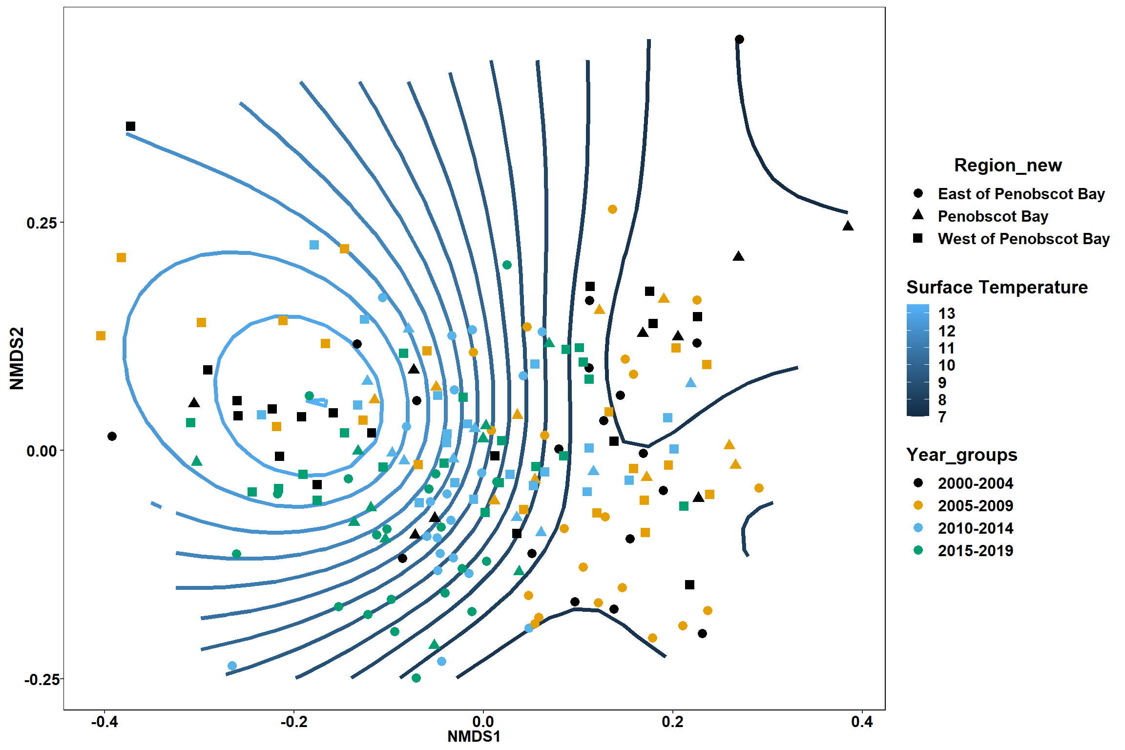
p1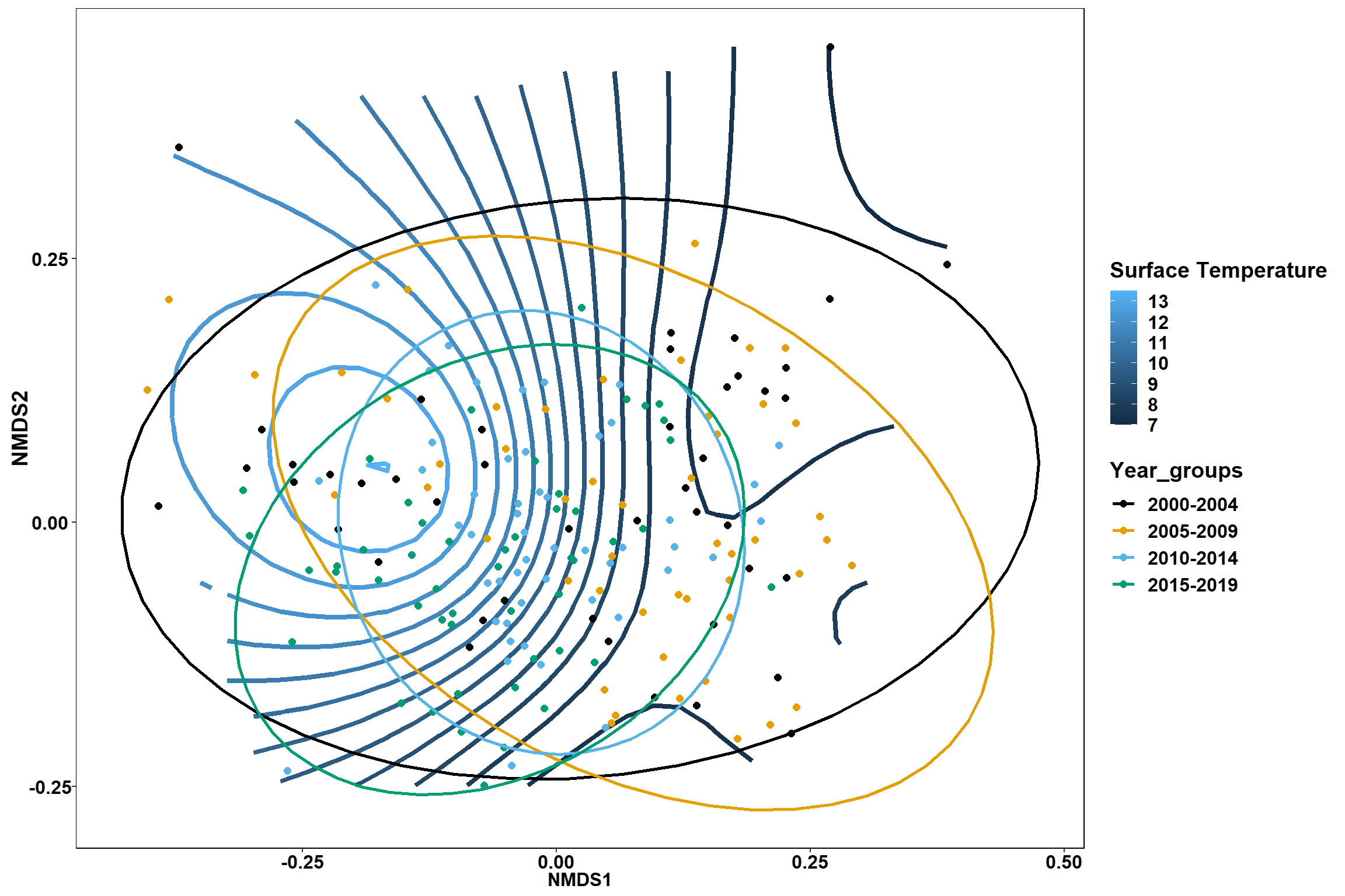
p2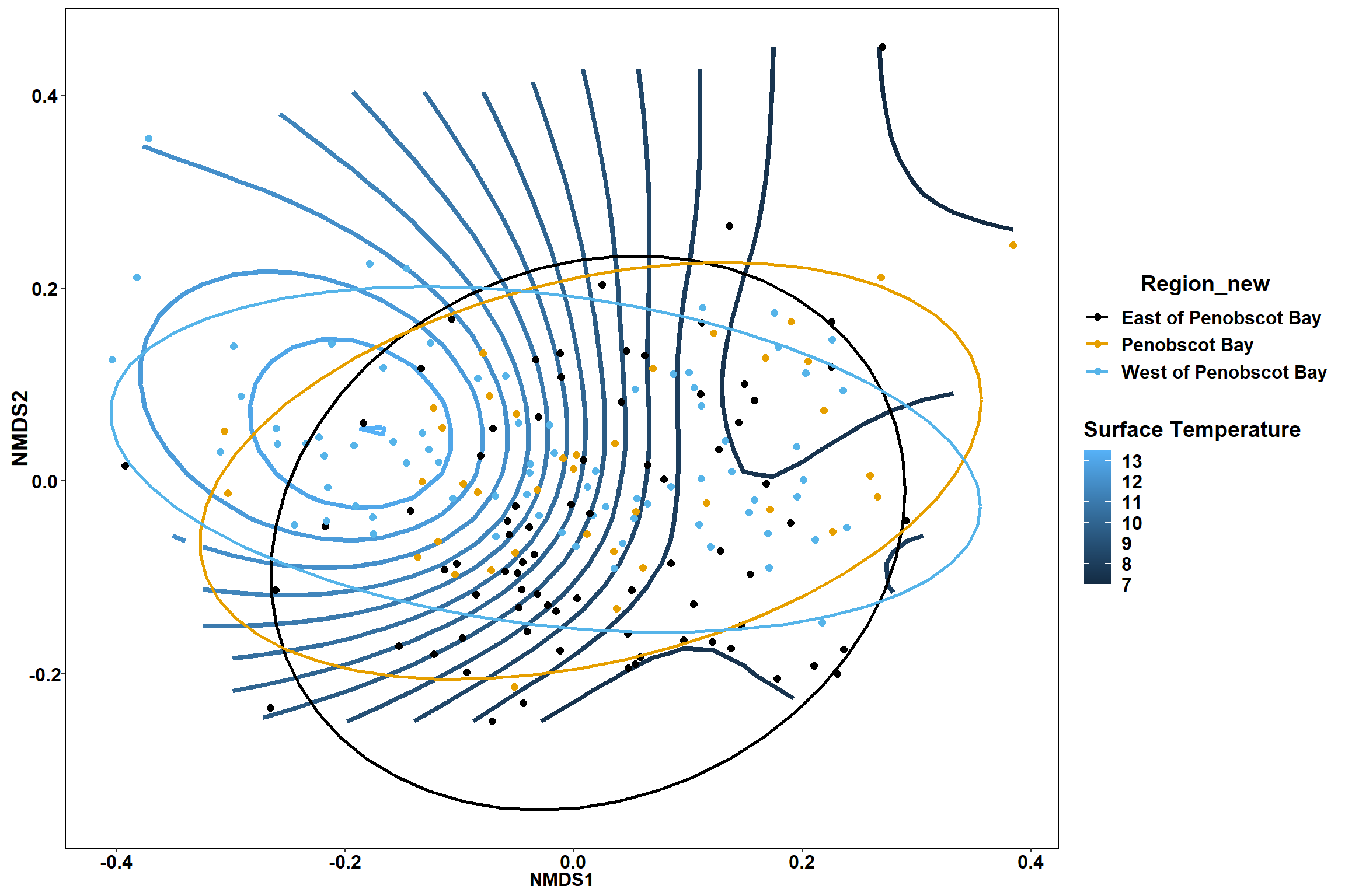
Bottom salinity
bottom_sal<-ordisurf(nmds, env$bottom_sal)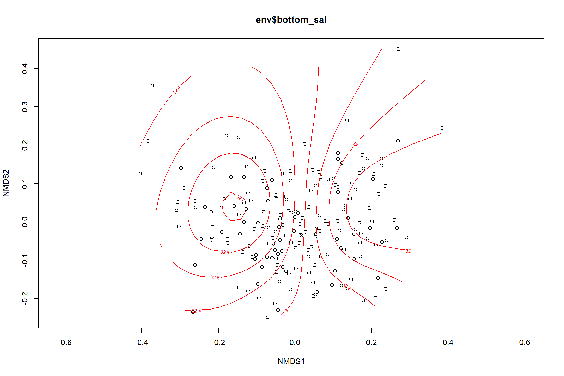
summary(bottom_sal)##
## Family: gaussian
## Link function: identity
##
## Formula:
## y ~ s(x1, x2, k = 10, bs = "tp", fx = FALSE)
##
## Parametric coefficients:
## Estimate Std. Error t value Pr(>|t|)
## (Intercept) 32.33134 0.03265 990.2 <2e-16 ***
## ---
## Signif. codes: 0 '***' 0.001 '**' 0.01 '*' 0.05 '.' 0.1 ' ' 1
##
## Approximate significance of smooth terms:
## edf Ref.df F p-value
## s(x1,x2) 5.029 9 6.363 <2e-16 ***
## ---
## Signif. codes: 0 '***' 0.001 '**' 0.01 '*' 0.05 '.' 0.1 ' ' 1
##
## R-sq.(adj) = 0.233 Deviance explained = 25.3%
## -REML = 125.2 Scale est. = 0.20256 n = 190ordi.grid <- bottom_sal$grid #extracts the ordisurf object
#str(ordi.grid) #it's a list though - cannot be plotted as is
ordi.mite <- expand.grid(x = ordi.grid$x, y = ordi.grid$y) #get x and ys
ordi.mite$z <- as.vector(ordi.grid$z) #unravel the matrix for the z scores
contour.vals <- data.frame(na.omit(ordi.mite)) #gets rid of the nas
p <- ggplot()+
stat_contour(data = contour.vals, aes(x, y, z=z, color = ..level..),position="identity",size=1.5)+
labs(x = "NMDS1", y = "NMDS2", color="Bottom Salinity")+
new_scale_color()+
geom_point(data = data.scores, aes(NMDS1, NMDS2, color=Year_groups, shape=Region_new), size = 3 )+ scale_color_colorblind()
p1 <- ggplot()+
stat_contour(data = contour.vals, aes(x, y, z=z, color = ..level..),position="identity",size=1.5)+
labs(x = "NMDS1", y = "NMDS2", color="Bottom Salinity")+
new_scale_color()+
geom_point(data = data.scores, aes(NMDS1, NMDS2, color=Year_groups), size = 2 )+ stat_ellipse(data=data.scores, aes(x=NMDS1, y=NMDS2, color=Year_groups),level = 0.95,size=1)+
scale_color_colorblind()
p2 <- ggplot()+
stat_contour(data = contour.vals, aes(x, y, z=z, color = ..level..),position="identity",size=1.5)+
labs(x = "NMDS1", y = "NMDS2", color="Bottom Salinity")+
new_scale_color()+
geom_point(data = data.scores, aes(NMDS1, NMDS2, color=Region_new), size = 2 )+stat_ellipse(data=data.scores, aes(x=NMDS1, y=NMDS2, color=Region_new),level = 0.95,size=1)+
scale_color_colorblind()
p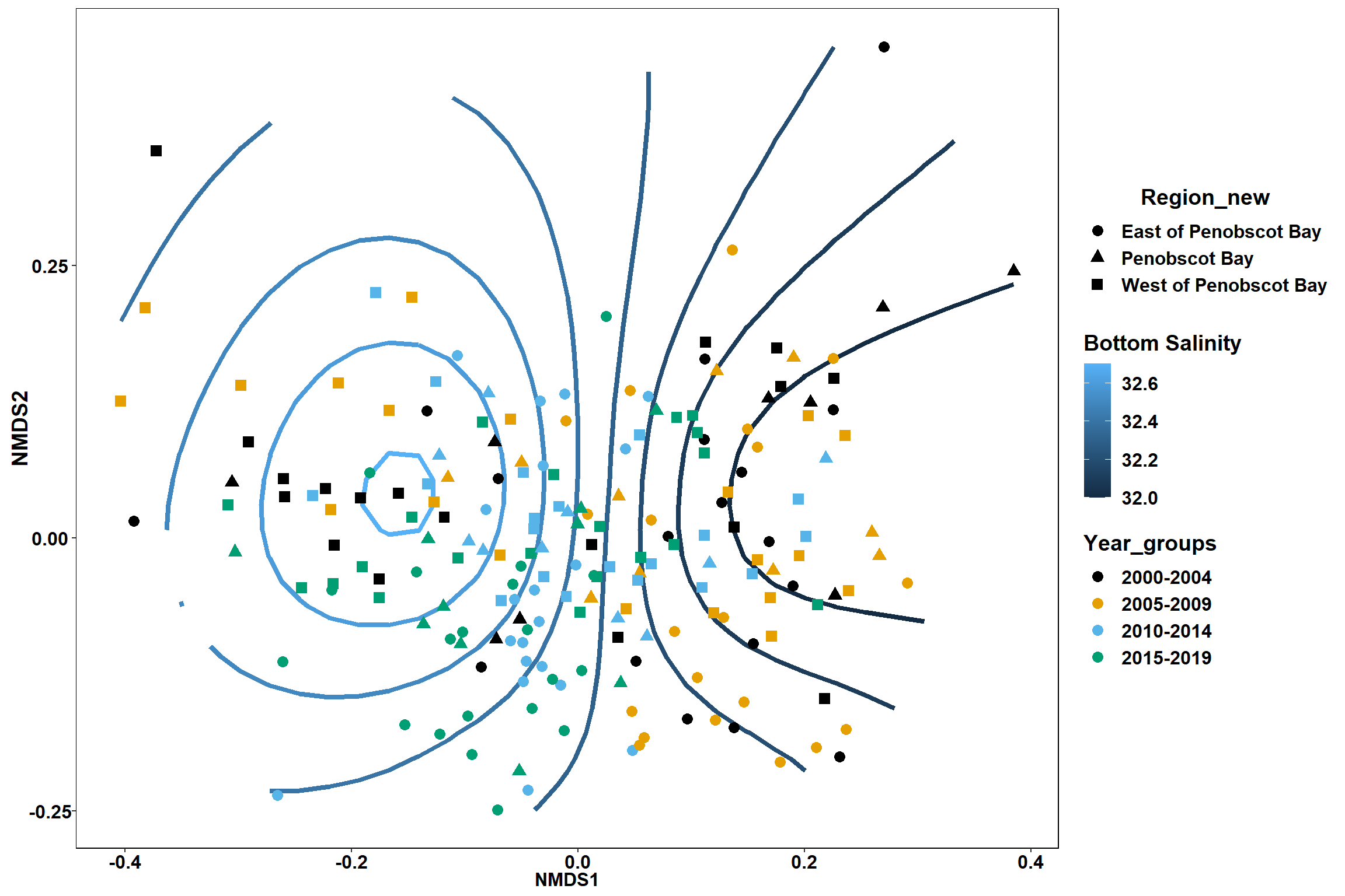
p1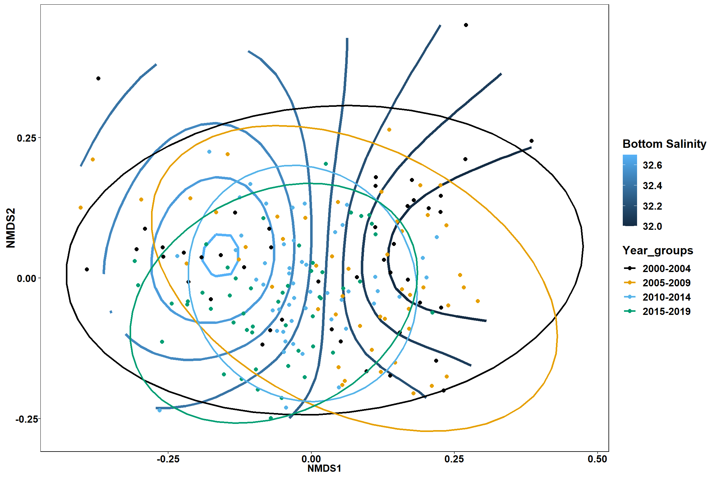
p2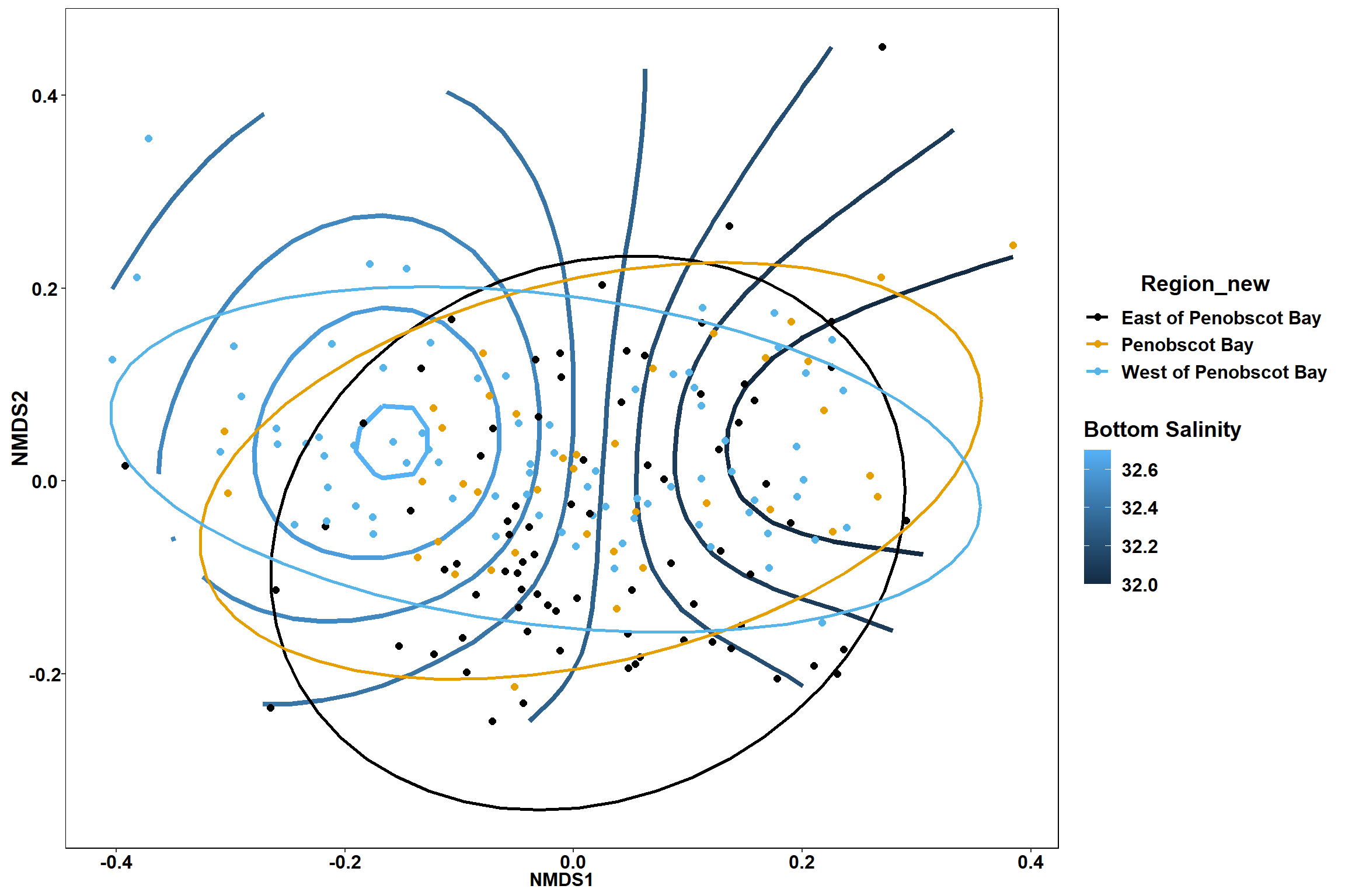
Surface salinity
surface_sal<-ordisurf(nmds, env$surface_sal)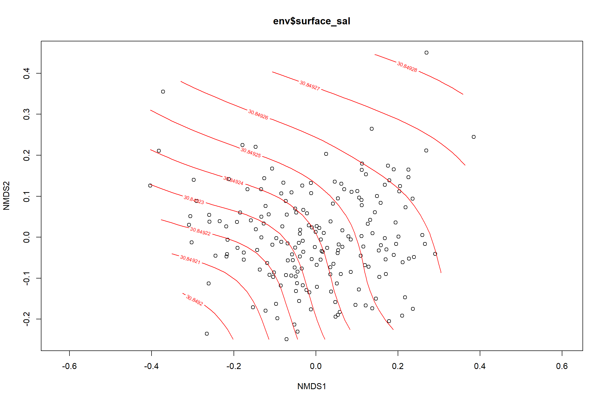
summary(surface_sal)##
## Family: gaussian
## Link function: identity
##
## Formula:
## y ~ s(x1, x2, k = 10, bs = "tp", fx = FALSE)
##
## Parametric coefficients:
## Estimate Std. Error t value Pr(>|t|)
## (Intercept) 30.8492 0.2342 131.7 <2e-16 ***
## ---
## Signif. codes: 0 '***' 0.001 '**' 0.01 '*' 0.05 '.' 0.1 ' ' 1
##
## Approximate significance of smooth terms:
## edf Ref.df F p-value
## s(x1,x2) 0.0003495 9 0 0.947
##
## R-sq.(adj) = -1.22e-06 Deviance explained = 6.28e-05%
## -REML = 492.33 Scale est. = 10.425 n = 190ordi.grid <- surface_sal$grid #extracts the ordisurf object
#str(ordi.grid) #it's a list though - cannot be plotted as is
ordi.mite <- expand.grid(x = ordi.grid$x, y = ordi.grid$y) #get x and ys
ordi.mite$z <- as.vector(ordi.grid$z) #unravel the matrix for the z scores
contour.vals <- data.frame(na.omit(ordi.mite)) #gets rid of the nas
p <- ggplot()+
stat_contour(data = contour.vals, aes(x, y, z=z, color = ..level..),position="identity",size=1.5)+
labs(x = "NMDS1", y = "NMDS2", color="Surface Salinity")+
new_scale_color()+
geom_point(data = data.scores, aes(NMDS1, NMDS2, color=Year_groups, shape=Region_new), size = 3 )+ scale_color_colorblind()
p1 <- ggplot()+
stat_contour(data = contour.vals, aes(x, y, z=z, color = ..level..),position="identity",size=1.5)+
labs(x = "NMDS1", y = "NMDS2", color="Surface Salinity")+
new_scale_color()+
geom_point(data = data.scores, aes(NMDS1, NMDS2, color=Year_groups), size = 2 )+stat_ellipse(data=data.scores, aes(x=NMDS1, y=NMDS2, color=Year_groups),level = 0.95,size=1)+
scale_color_colorblind()
p2 <- ggplot()+
stat_contour(data = contour.vals, aes(x, y, z=z, color = ..level..),position="identity",size=1.5)+
labs(x = "NMDS1", y = "NMDS2", color="Surface Salinity")+
new_scale_color()+
geom_point(data = data.scores, aes(NMDS1, NMDS2, color=Region_new), size = 2 )+stat_ellipse(data=data.scores, aes(x=NMDS1, y=NMDS2, color=Region_new),level = 0.95,size=1)+
scale_color_colorblind()
p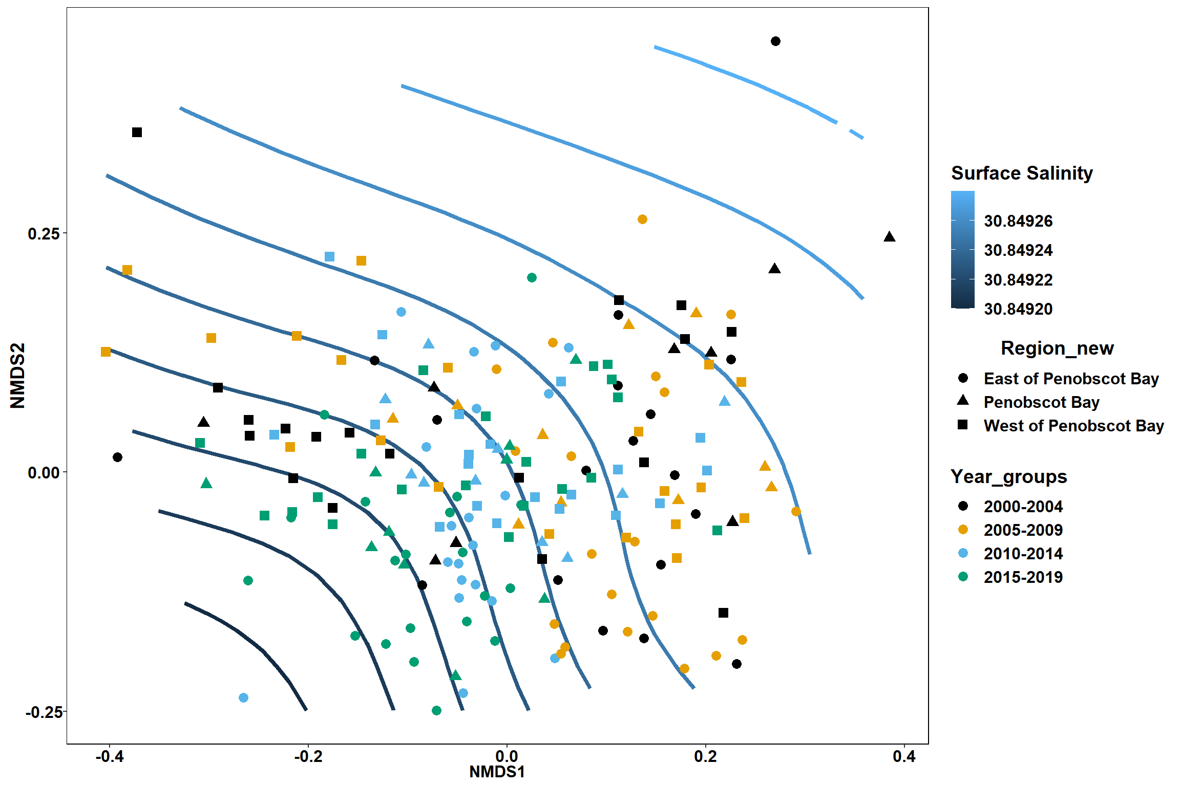
p1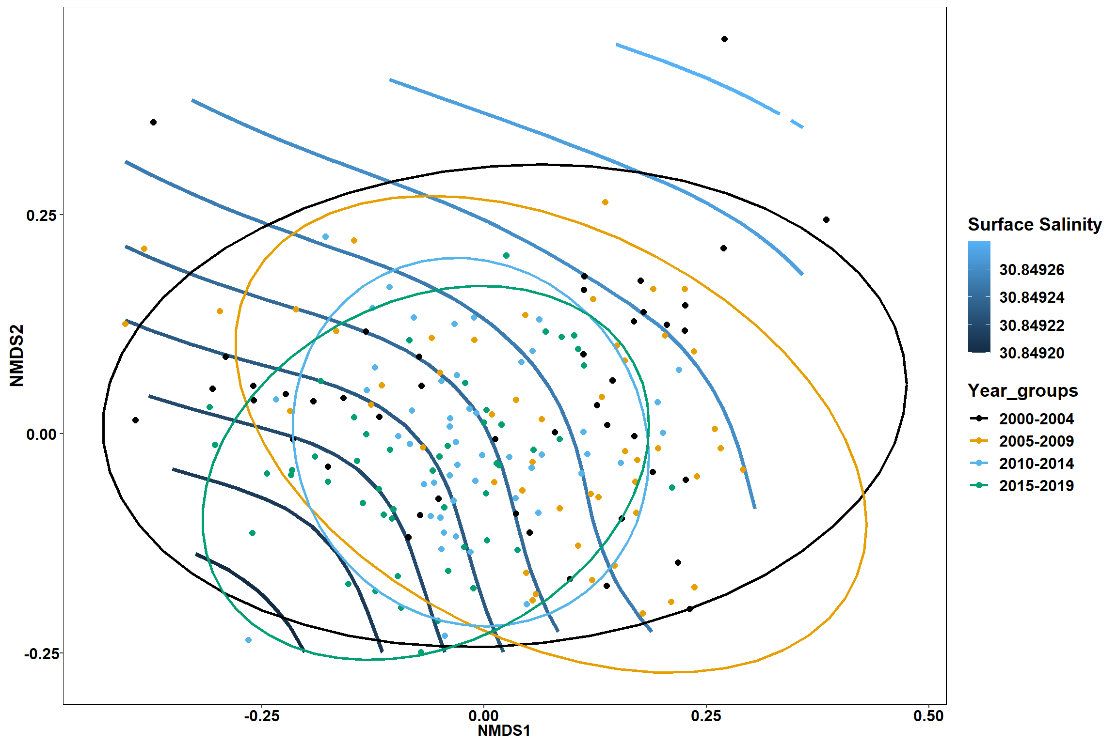
p2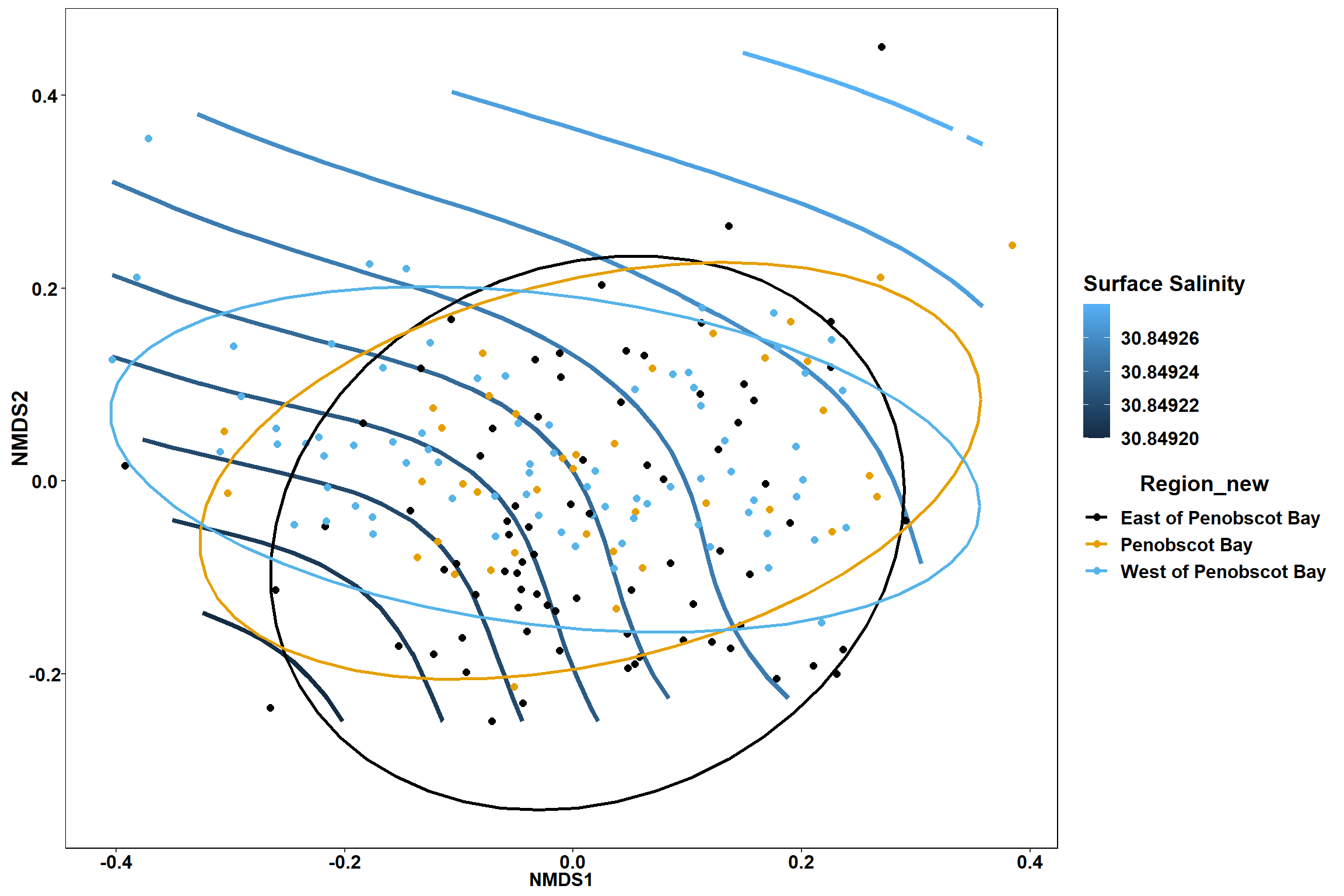
start latitude
start_lat<-ordisurf(nmds, env$start_lat)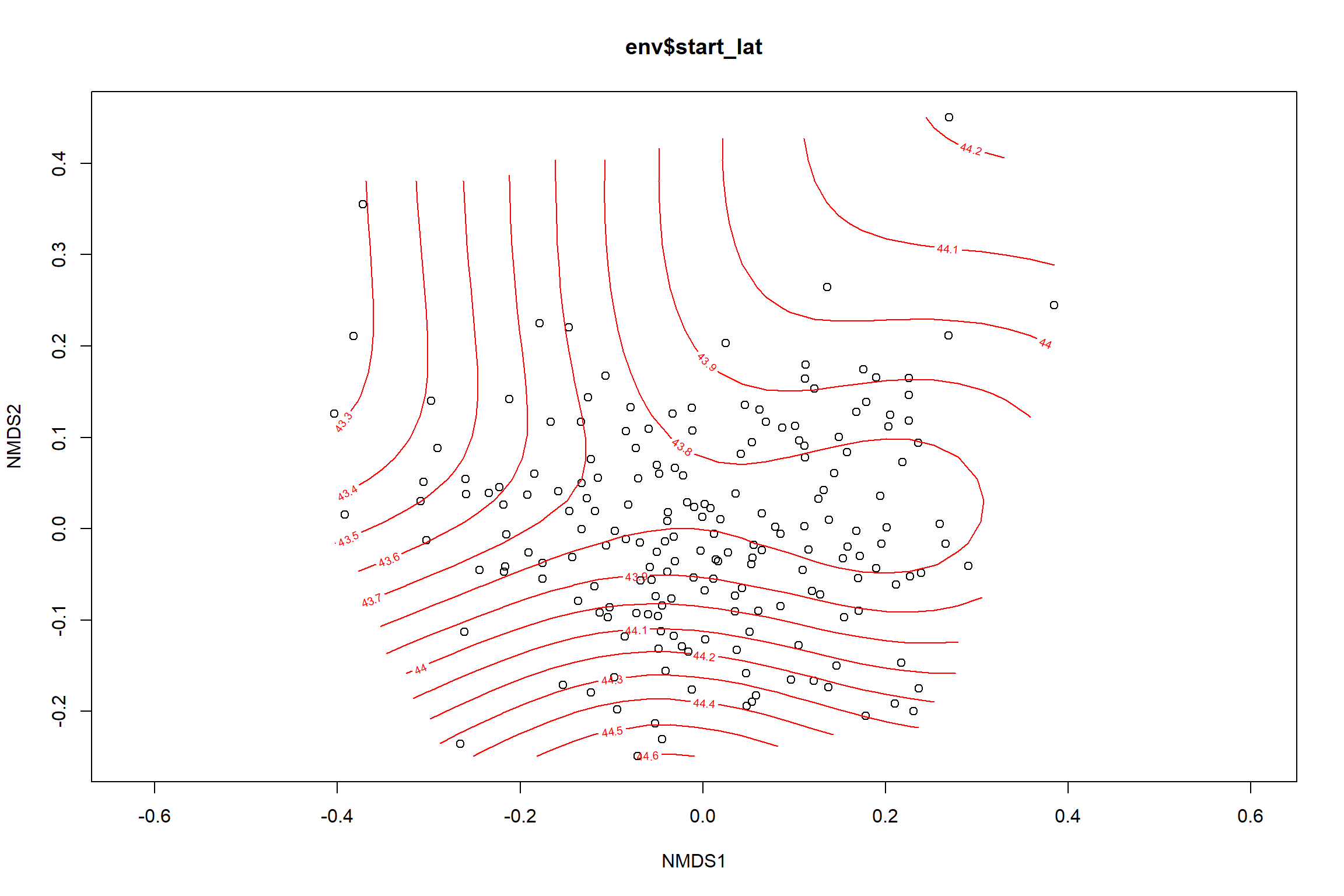
summary(start_lat)##
## Family: gaussian
## Link function: identity
##
## Formula:
## y ~ s(x1, x2, k = 10, bs = "tp", fx = FALSE)
##
## Parametric coefficients:
## Estimate Std. Error t value Pr(>|t|)
## (Intercept) 43.87499 0.02602 1687 <2e-16 ***
## ---
## Signif. codes: 0 '***' 0.001 '**' 0.01 '*' 0.05 '.' 0.1 ' ' 1
##
## Approximate significance of smooth terms:
## edf Ref.df F p-value
## s(x1,x2) 7.37 9 8.919 <2e-16 ***
## ---
## Signif. codes: 0 '***' 0.001 '**' 0.01 '*' 0.05 '.' 0.1 ' ' 1
##
## R-sq.(adj) = 0.293 Deviance explained = 32%
## -REML = 91.074 Scale est. = 0.13198 n = 195ordi.grid <- start_lat$grid #extracts the ordisurf object
#str(ordi.grid) #it's a list though - cannot be plotted as is
ordi.mite <- expand.grid(x = ordi.grid$x, y = ordi.grid$y) #get x and ys
ordi.mite$z <- as.vector(ordi.grid$z) #unravel the matrix for the z scores
contour.vals <- data.frame(na.omit(ordi.mite)) #gets rid of the nas
p <- ggplot()+
stat_contour(data = contour.vals, aes(x, y, z=z, color = ..level..),position="identity",size=1.5)+
labs(x = "NMDS1", y = "NMDS2", color="Latitude")+
new_scale_color()+
geom_point(data = data.scores, aes(NMDS1, NMDS2, color=Year_groups, shape=Region_new), size = 3 )+ scale_color_colorblind()
p1 <- ggplot()+
stat_contour(data = contour.vals, aes(x, y, z=z, color = ..level..),position="identity",size=1.5)+
labs(x = "NMDS1", y = "NMDS2", color="Latitude")+
new_scale_color()+
geom_point(data = data.scores, aes(NMDS1, NMDS2, color=Year_groups), size = 2 )+ stat_ellipse(data=data.scores, aes(x=NMDS1, y=NMDS2, color=Year_groups),level = 0.95,size=1)+
scale_color_colorblind()
p2 <- ggplot()+
stat_contour(data = contour.vals, aes(x, y, z=z, color = ..level..),position="identity",size=1.5)+
labs(x = "NMDS1", y = "NMDS2", color="Latitude")+
new_scale_color()+
geom_point(data = data.scores, aes(NMDS1, NMDS2, color=Region_new), size = 2 )+ stat_ellipse(data=data.scores, aes(x=NMDS1, y=NMDS2, color=Region_new),level = 0.95,size=1)+
scale_color_colorblind()
p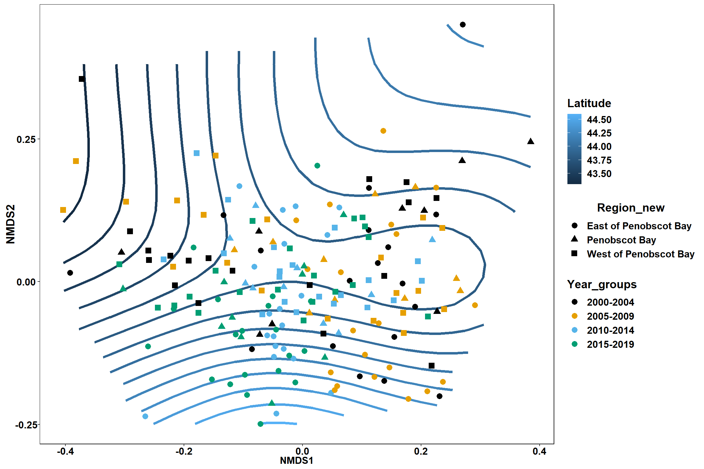
p1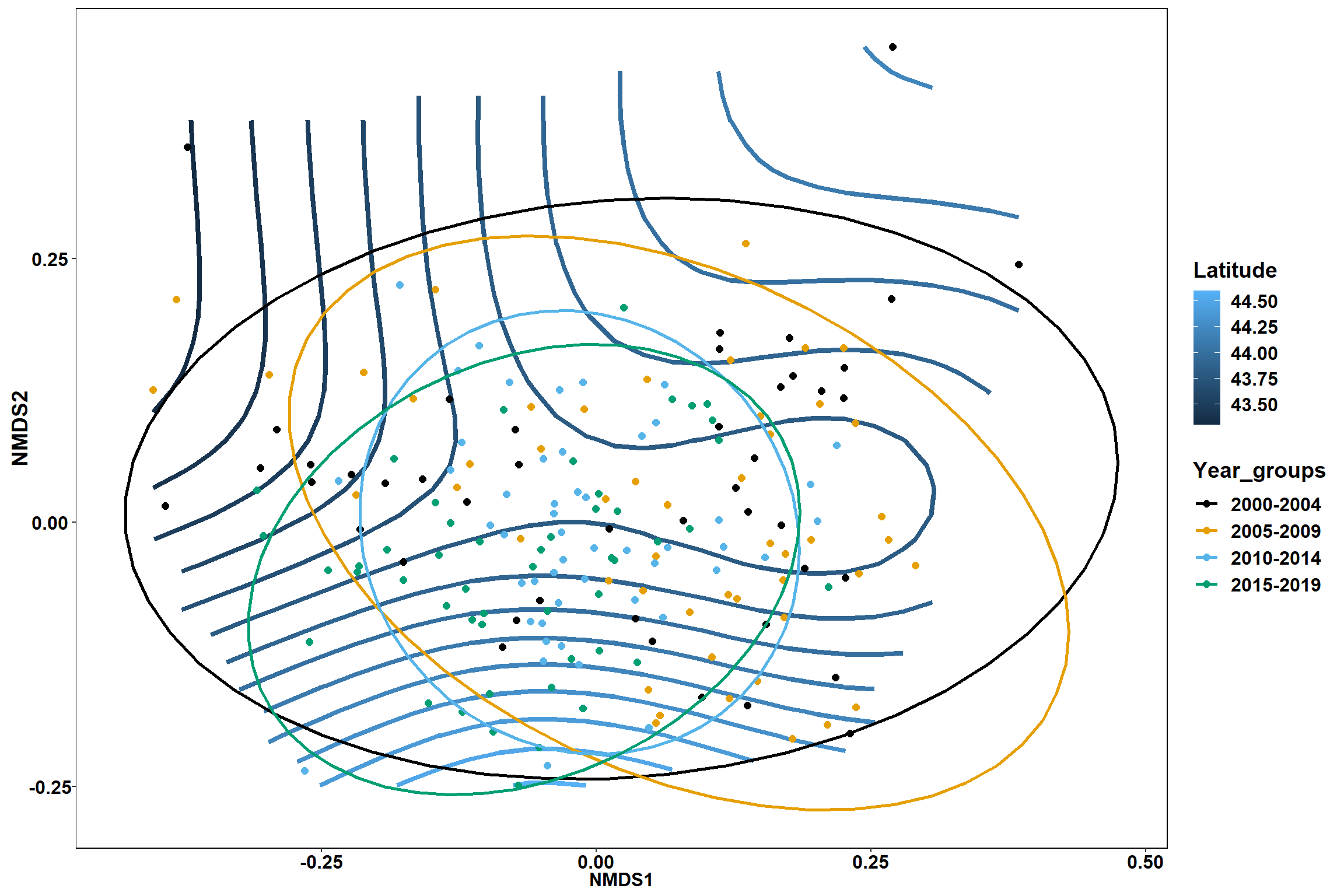
p2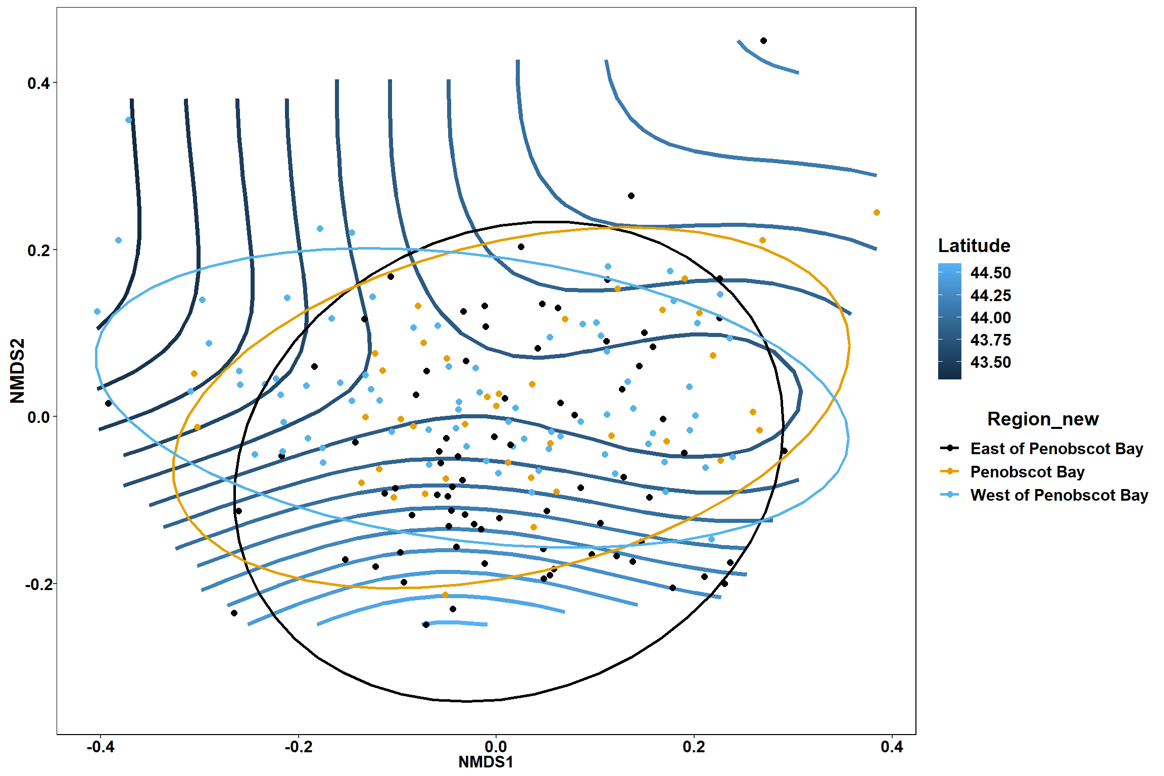
start longitude
start_long<-ordisurf(nmds, env$start_long)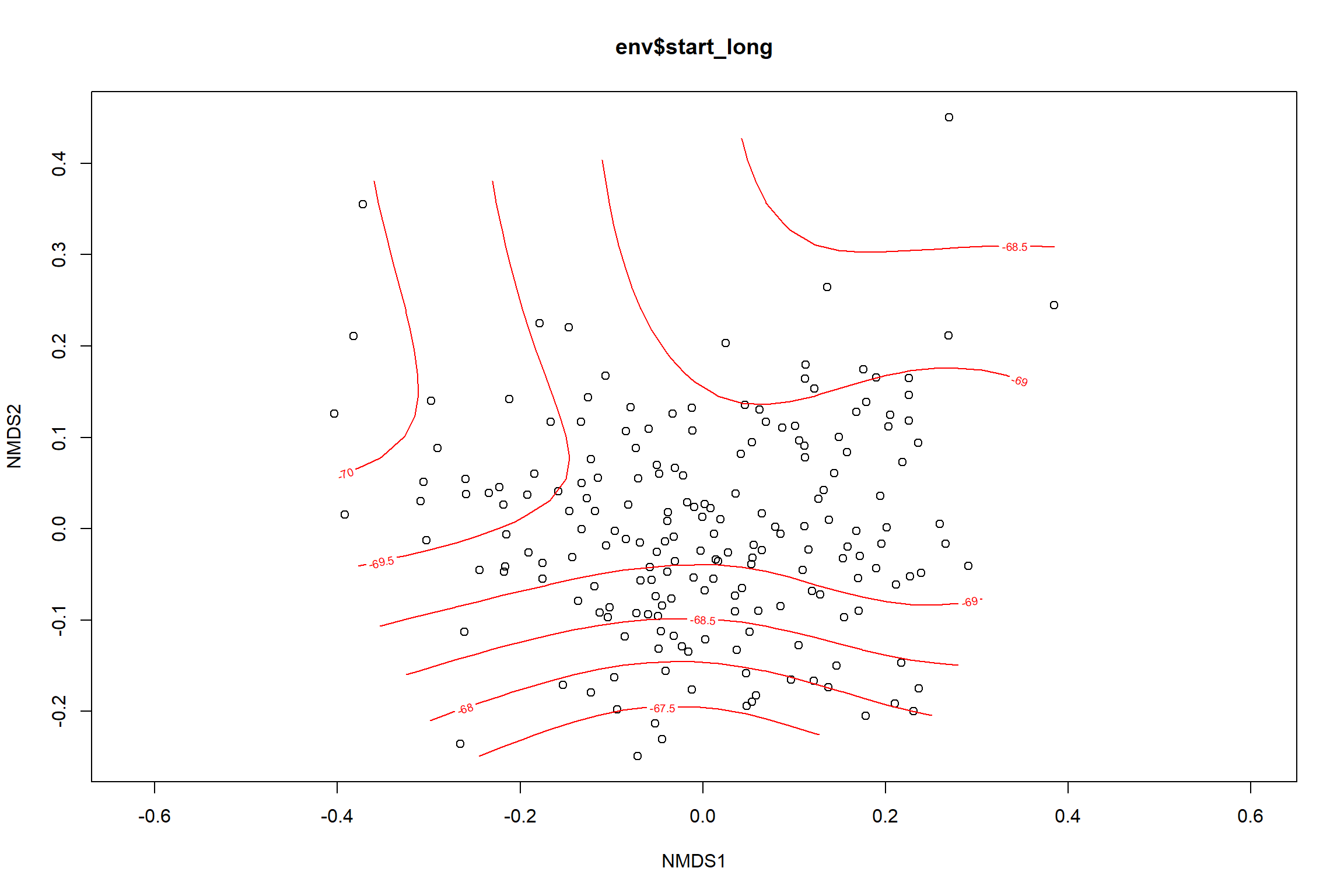
summary(start_long)##
## Family: gaussian
## Link function: identity
##
## Formula:
## y ~ s(x1, x2, k = 10, bs = "tp", fx = FALSE)
##
## Parametric coefficients:
## Estimate Std. Error t value Pr(>|t|)
## (Intercept) -68.97337 0.06034 -1143 <2e-16 ***
## ---
## Signif. codes: 0 '***' 0.001 '**' 0.01 '*' 0.05 '.' 0.1 ' ' 1
##
## Approximate significance of smooth terms:
## edf Ref.df F p-value
## s(x1,x2) 7.539 9 10.6 <2e-16 ***
## ---
## Signif. codes: 0 '***' 0.001 '**' 0.01 '*' 0.05 '.' 0.1 ' ' 1
##
## R-sq.(adj) = 0.33 Deviance explained = 35.6%
## -REML = 254.73 Scale est. = 0.70989 n = 195ordi.grid <- start_long$grid #extracts the ordisurf object
#str(ordi.grid) #it's a list though - cannot be plotted as is
ordi.mite <- expand.grid(x = ordi.grid$x, y = ordi.grid$y) #get x and ys
ordi.mite$z <- as.vector(ordi.grid$z) #unravel the matrix for the z scores
contour.vals <- data.frame(na.omit(ordi.mite)) #gets rid of the nas
p <- ggplot()+
stat_contour(data = contour.vals, aes(x, y, z=z, color = ..level..),position="identity",size=1.5)+
labs(x = "NMDS1", y = "NMDS2", color="Longitude")+
new_scale_color()+
geom_point(data = data.scores, aes(NMDS1, NMDS2, color=Year_groups, shape=Region_new), size = 3 )+ scale_color_colorblind()
p1 <- ggplot()+
stat_contour(data = contour.vals, aes(x, y, z=z, color = ..level..),position="identity",size=1.5)+
labs(x = "NMDS1", y = "NMDS2", color="Longitude")+
new_scale_color()+
geom_point(data = data.scores, aes(NMDS1, NMDS2, color=Year_groups), size = 2 )+stat_ellipse(data=data.scores, aes(x=NMDS1, y=NMDS2, color=Year_groups),level = 0.95,size=1)+
scale_color_colorblind()
p2 <- ggplot()+
stat_contour(data = contour.vals, aes(x, y, z=z, color = ..level..),position="identity",size=1.5)+
labs(x = "NMDS1", y = "NMDS2", color="Longitude")+
new_scale_color()+
geom_point(data = data.scores, aes(NMDS1, NMDS2, color=Region_new), size = 2 )+stat_ellipse(data=data.scores, aes(x=NMDS1, y=NMDS2, color=Region_new),level = 0.95,size=1)+
scale_color_colorblind()
p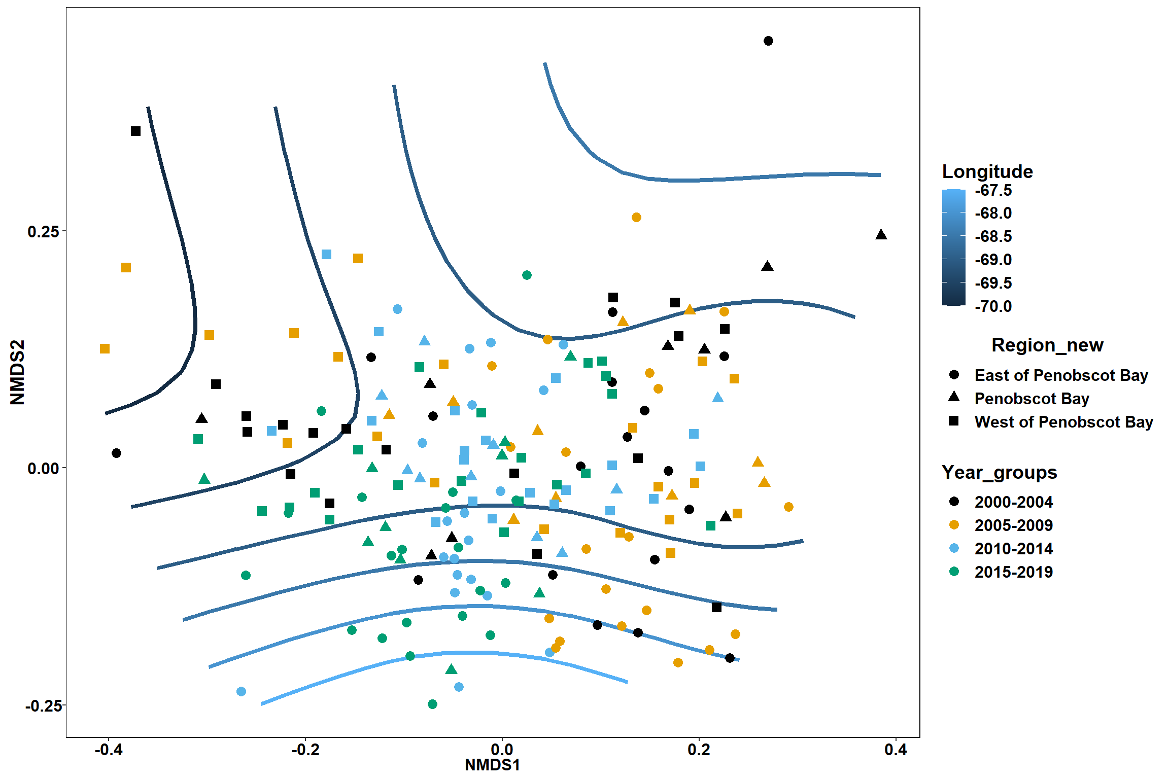
p1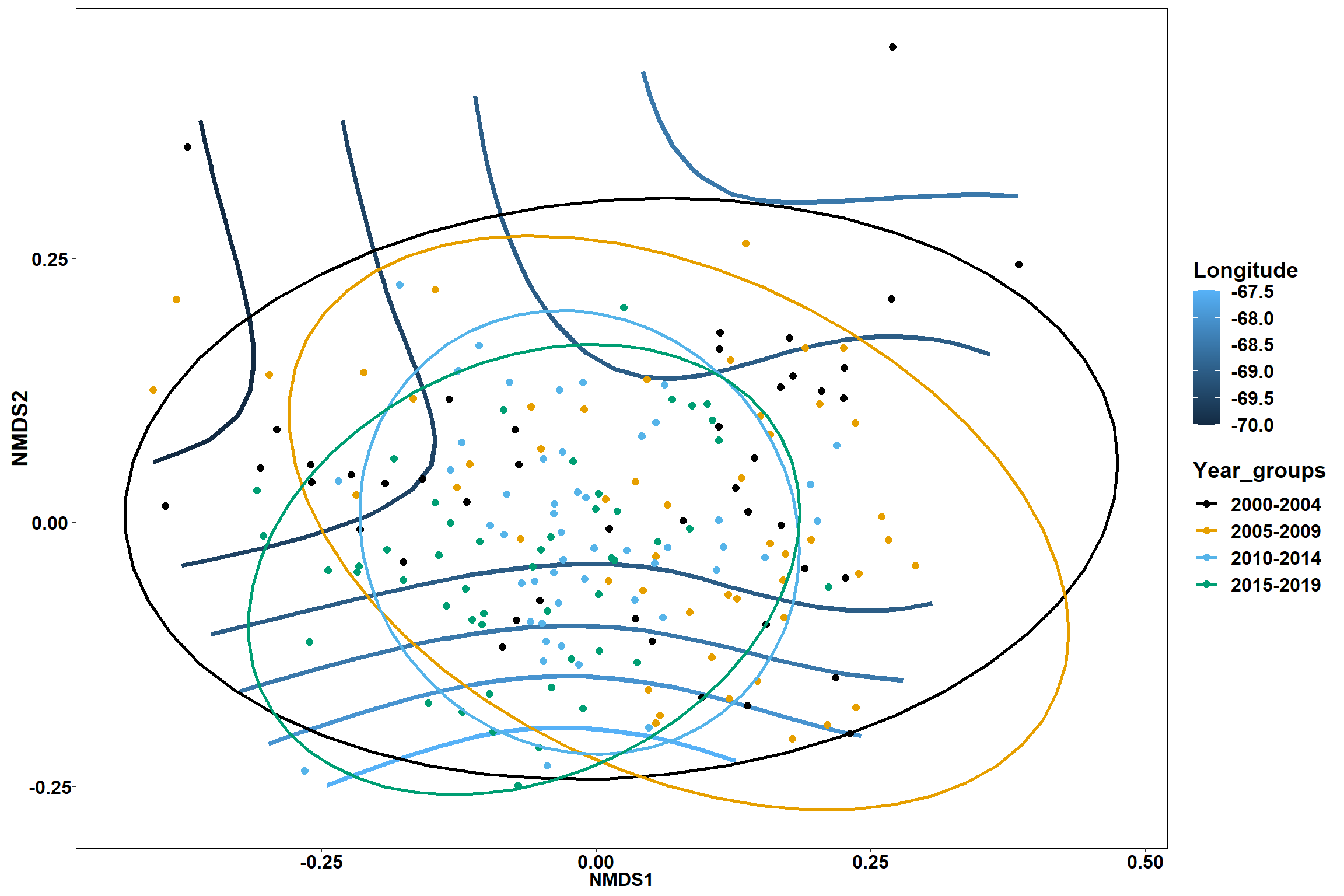
p2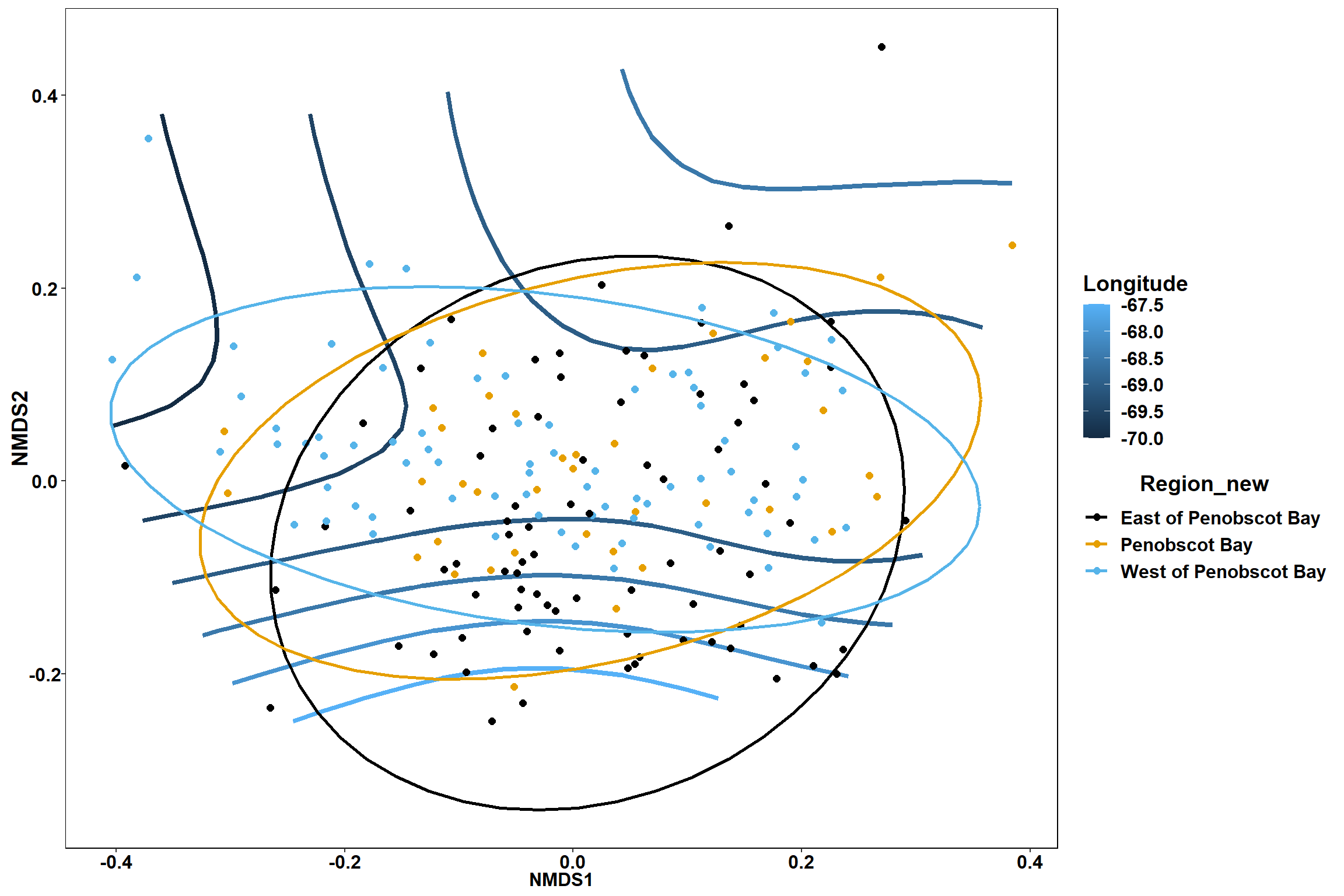
start depth
start_depth<-ordisurf(nmds, env$start_depth)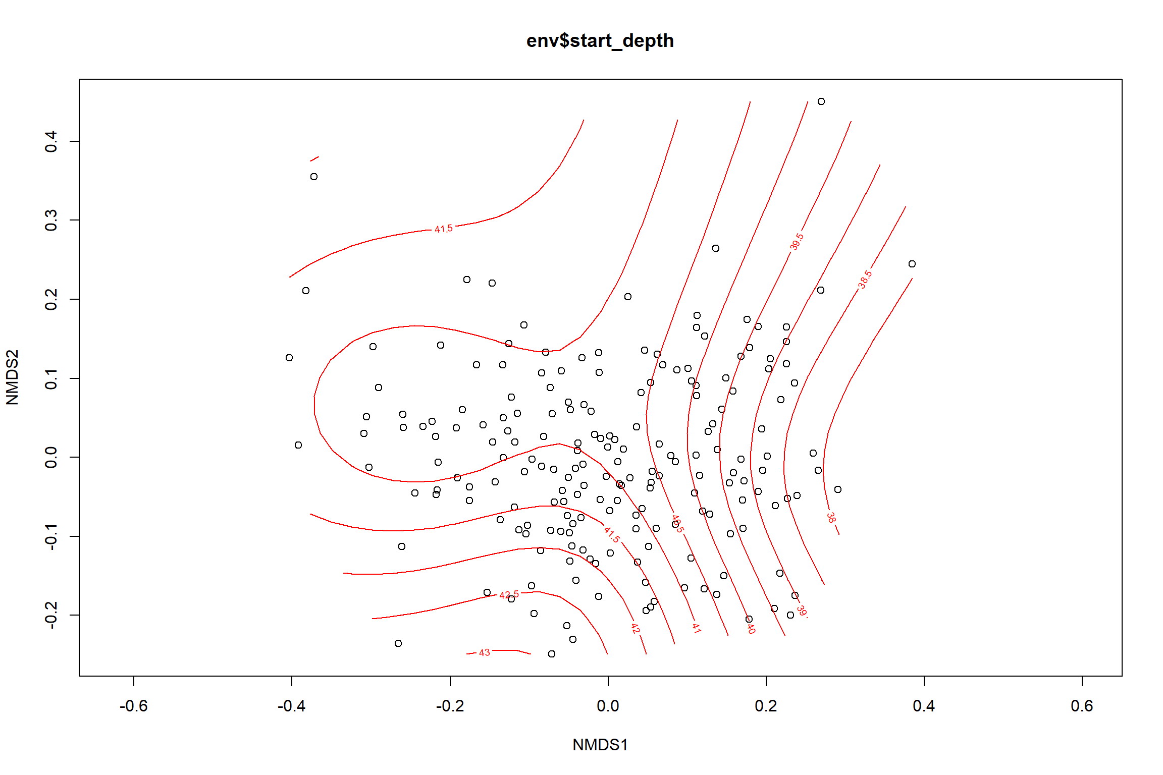
summary(start_depth)##
## Family: gaussian
## Link function: identity
##
## Formula:
## y ~ s(x1, x2, k = 10, bs = "tp", fx = FALSE)
##
## Parametric coefficients:
## Estimate Std. Error t value Pr(>|t|)
## (Intercept) 40.6472 0.3104 130.9 <2e-16 ***
## ---
## Signif. codes: 0 '***' 0.001 '**' 0.01 '*' 0.05 '.' 0.1 ' ' 1
##
## Approximate significance of smooth terms:
## edf Ref.df F p-value
## s(x1,x2) 4.618 9 1.703 0.0027 **
## ---
## Signif. codes: 0 '***' 0.001 '**' 0.01 '*' 0.05 '.' 0.1 ' ' 1
##
## R-sq.(adj) = 0.0732 Deviance explained = 9.53%
## -REML = 566.64 Scale est. = 18.794 n = 195ordi.grid <- start_depth$grid #extracts the ordisurf object
#str(ordi.grid) #it's a list though - cannot be plotted as is
ordi.mite <- expand.grid(x = ordi.grid$x, y = ordi.grid$y) #get x and ys
ordi.mite$z <- as.vector(ordi.grid$z) #unravel the matrix for the z scores
contour.vals <- data.frame(na.omit(ordi.mite)) #gets rid of the nas
p <- ggplot()+
stat_contour(data = contour.vals, aes(x, y, z=z, color = ..level..),position="identity",size=1.5)+
labs(x = "NMDS1", y = "NMDS2", color="Depth")+
new_scale_color()+
geom_point(data = data.scores, aes(NMDS1, NMDS2, color=Year_groups, shape=Region_new), size = 3 )+ scale_color_colorblind()
p1 <- ggplot()+
stat_contour(data = contour.vals, aes(x, y, z=z, color = ..level..),position="identity",size=1.5)+
labs(x = "NMDS1", y = "NMDS2", color="Depth")+
new_scale_color()+
geom_point(data = data.scores, aes(NMDS1, NMDS2, color=Year_groups), size = 2 )+stat_ellipse(data=data.scores, aes(x=NMDS1, y=NMDS2, color=Year_groups),level = 0.95,size=1)+
scale_color_colorblind()
p2 <- ggplot()+
stat_contour(data = contour.vals, aes(x, y, z=z, color = ..level..),position="identity",size=1.5)+
labs(x = "NMDS1", y = "NMDS2", color="Depth")+
new_scale_color()+
geom_point(data = data.scores, aes(NMDS1, NMDS2, color=Region_new), size = 2 )+stat_ellipse(data=data.scores, aes(x=NMDS1, y=NMDS2, color=Region_new),level = 0.95,size=1)+
scale_color_colorblind()
p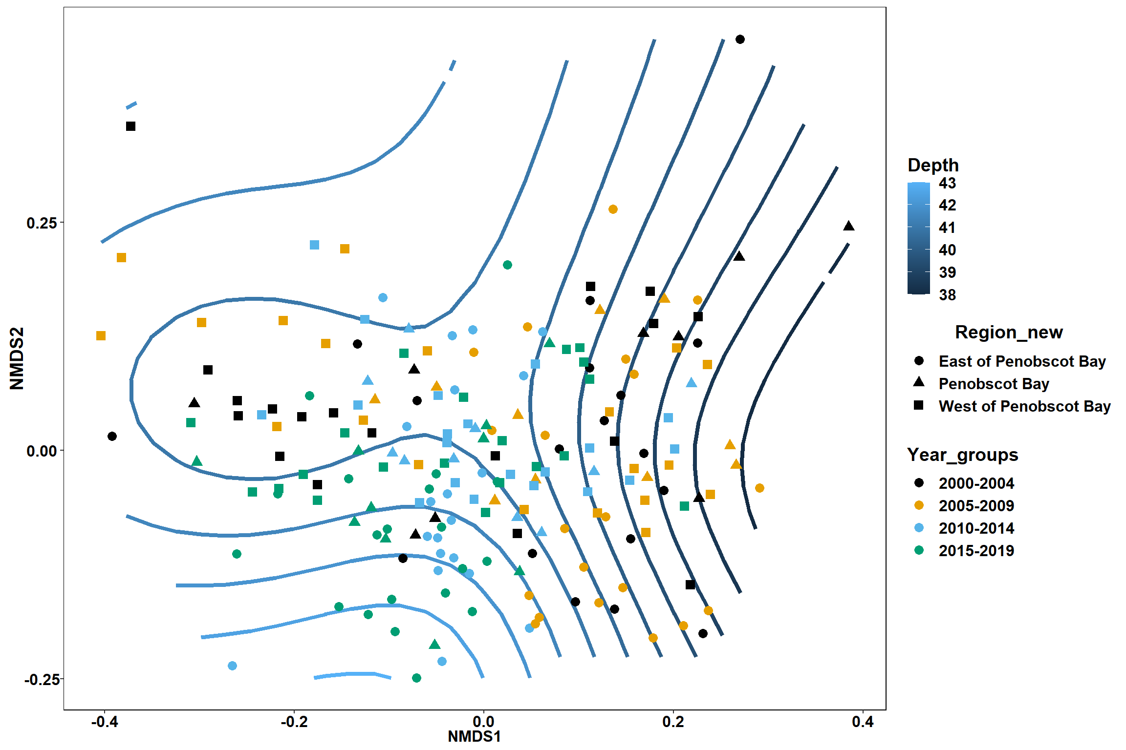
p1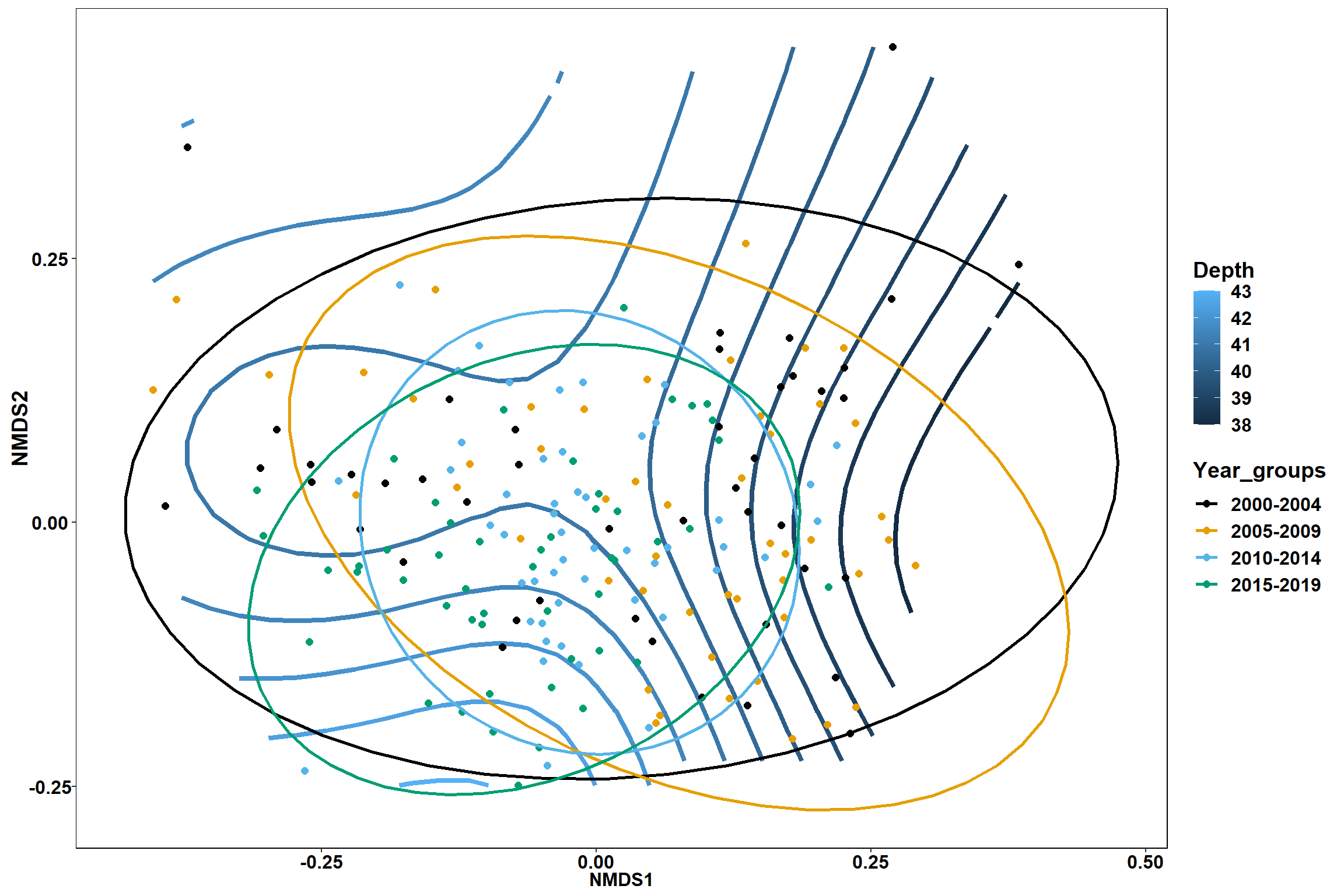
p2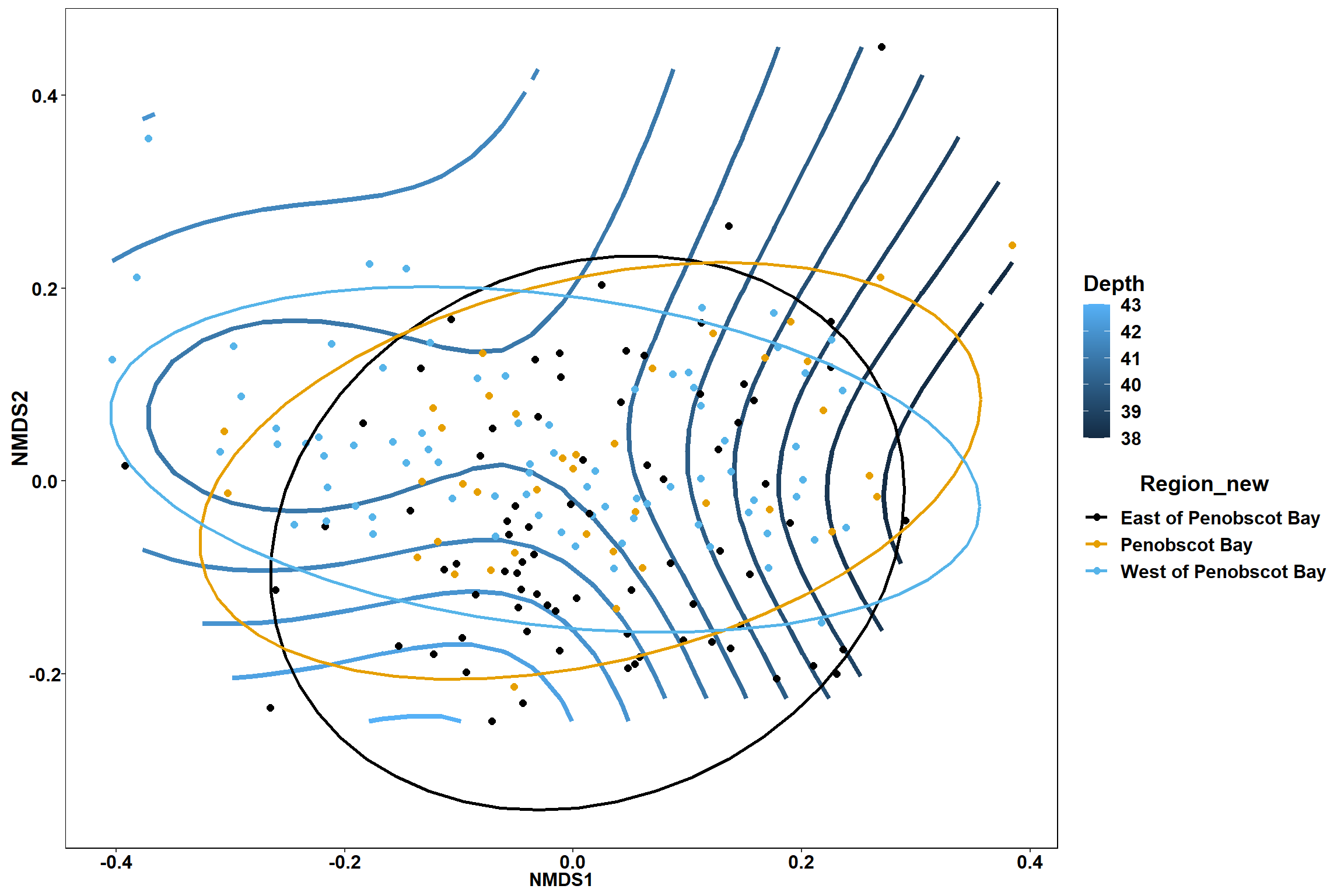
Top 50 Species Biomass
NMDS
#load in data
trawl_data_arrange<-read.csv(here("Data/species_biomass_matrix.csv"))[-1]

trawl_data<-read.csv(here("Data/MaineDMR_Trawl_Survey_Tow_Data_2021-05-14.csv"))

all_Data<-group_by(trawl_data, Season, Year, Region)%>%
  filter(Year<2020)%>%
  summarise(start_lat=mean(Start_Latitude),start_long=mean(Start_Longitude),end_lat=mean(End_Latitude), end_long=mean(End_Longitude),start_depth=mean(Start_Depth_fathoms, na.rm=TRUE), end_depth=mean(End_Depth_fathoms, na.rm=TRUE), bottom_temp=mean(Bottom_WaterTemp_DegC, na.rm=TRUE), bottom_sal=mean(Bottom_Salinity, na.rm=TRUE),surface_temp=mean(Surface_WaterTemp_DegC, na.rm=TRUE), surface_sal=mean(Surface_Salinity, na.rm=TRUE))%>%
  full_join(trawl_data_arrange)%>%
  ungroup()

com<-select(all_Data, 14:63)

com<-vegdist(com, method="bray")

#convert com to a matrix
m_com = as.matrix(com)

set.seed(123)
nmds = metaMDS(m_com,k=2, distance = "bray", trymax = 500)
## Run 0 stress 0.2121976
## Run 1 stress 0.2129894
## Run 2 stress 0.2065891
## ... New best solution
## ... Procrustes: rmse 0.03066016 max resid 0.394017
## Run 3 stress 0.2321135
## Run 4 stress 0.2078851
## Run 5 stress 0.2068134
## ... Procrustes: rmse 0.02915097 max resid 0.2055298
## Run 6 stress 0.2127907
## Run 7 stress 0.2078697
## Run 8 stress 0.2061183
## ... New best solution
## ... Procrustes: rmse 0.01620476 max resid 0.2111533
## Run 9 stress 0.2063589
## ... Procrustes: rmse 0.01024384 max resid 0.1293444
## Run 10 stress 0.2065615
## ... Procrustes: rmse 0.01586056 max resid 0.2115795
## Run 11 stress 0.2057376
## ... New best solution
## ... Procrustes: rmse 0.006280238 max resid 0.07403794
## Run 12 stress 0.2223293
## Run 13 stress 0.2061959
## ... Procrustes: rmse 0.01002217 max resid 0.08219748
## Run 14 stress 0.2061249
## ... Procrustes: rmse 0.007921465 max resid 0.07564778
## Run 15 stress 0.2078696
## Run 16 stress 0.2066023
## Run 17 stress 0.2078697
## Run 18 stress 0.2078724
## Run 19 stress 0.2129545
## Run 20 stress 0.2058355
## ... Procrustes: rmse 0.004467055 max resid 0.02821935
## Run 21 stress 0.2127013
## Run 22 stress 0.2058589
## ... Procrustes: rmse 0.007143827 max resid 0.04871218
## Run 23 stress 0.2090882
## Run 24 stress 0.2057963
## ... Procrustes: rmse 0.006359738 max resid 0.04886675
## Run 25 stress 0.2061198
## ... Procrustes: rmse 0.006030516 max resid 0.07288652
## Run 26 stress 0.2062534
## Run 27 stress 0.2078726
## Run 28 stress 0.2158658
## Run 29 stress 0.2078697
## Run 30 stress 0.2120911
## Run 31 stress 0.2118629
## Run 32 stress 0.2136581
## Run 33 stress 0.2061525
## ... Procrustes: rmse 0.006968232 max resid 0.07723316
## Run 34 stress 0.2121226
## Run 35 stress 0.2127652
## Run 36 stress 0.2080182
## Run 37 stress 0.2250331
## Run 38 stress 0.2065819
## Run 39 stress 0.2061254
## ... Procrustes: rmse 0.007985836 max resid 0.07619115
## Run 40 stress 0.2065615
## Run 41 stress 0.2124912
## Run 42 stress 0.2061197
## ... Procrustes: rmse 0.006355229 max resid 0.07480883
## Run 43 stress 0.2068125
## Run 44 stress 0.2064923
## Run 45 stress 0.2090879
## Run 46 stress 0.2061809
## ... Procrustes: rmse 0.01100693 max resid 0.08288323
## Run 47 stress 0.2061184
## ... Procrustes: rmse 0.006293763 max resid 0.07425619
## Run 48 stress 0.2063299
## Run 49 stress 0.2147466
## Run 50 stress 0.206164
## ... Procrustes: rmse 0.00963397 max resid 0.1248158
## Run 51 stress 0.211741
## Run 52 stress 0.4165594
## Run 53 stress 0.2061961
## ... Procrustes: rmse 0.01004438 max resid 0.08220953
## Run 54 stress 0.2061094
## ... Procrustes: rmse 0.006083115 max resid 0.07283369
## Run 55 stress 0.2061256
## ... Procrustes: rmse 0.008030977 max resid 0.07652824
## Run 56 stress 0.2090879
## Run 57 stress 0.2211213
## Run 58 stress 0.2068131
## Run 59 stress 0.2217395
## Run 60 stress 0.2127076
## Run 61 stress 0.2061307
## ... Procrustes: rmse 0.009372368 max resid 0.1243742
## Run 62 stress 0.2061229
## ... Procrustes: rmse 0.009878406 max resid 0.123909
## Run 63 stress 0.2065852
## Run 64 stress 0.2063197
## Run 65 stress 0.2126293
## Run 66 stress 0.2224418
## Run 67 stress 0.2090938
## Run 68 stress 0.2063816
## Run 69 stress 0.2065614
## Run 70 stress 0.2058137
## ... Procrustes: rmse 0.006205867 max resid 0.04862407
## Run 71 stress 0.2214504
## Run 72 stress 0.2078858
## Run 73 stress 0.2065614
## Run 74 stress 0.2068128
## Run 75 stress 0.2065985
## Run 76 stress 0.2078725
## Run 77 stress 0.2065513
## Run 78 stress 0.2113782
## Run 79 stress 0.2064735
## Run 80 stress 0.2209042
## Run 81 stress 0.2068126
## Run 82 stress 0.2066
## Run 83 stress 0.2117095
## Run 84 stress 0.2065997
## Run 85 stress 0.2113613
## Run 86 stress 0.2120856
## Run 87 stress 0.206463
## Run 88 stress 0.213848
## Run 89 stress 0.2068102
## Run 90 stress 0.2127135
## Run 91 stress 0.2090882
## Run 92 stress 0.2129931
## Run 93 stress 0.2078869
## Run 94 stress 0.2096572
## Run 95 stress 0.2062792
## Run 96 stress 0.2130205
## Run 97 stress 0.221723
## Run 98 stress 0.2063669
## Run 99 stress 0.2065615
## Run 100 stress 0.209088
## Run 101 stress 0.208019
## Run 102 stress 0.2065925
## Run 103 stress 0.2064454
## Run 104 stress 0.2126814
## Run 105 stress 0.2060862
## ... Procrustes: rmse 0.006689337 max resid 0.0720389
## Run 106 stress 0.2243925
## Run 107 stress 0.209088
## Run 108 stress 0.2057889
## ... Procrustes: rmse 0.005941908 max resid 0.04863602
## Run 109 stress 0.2117035
## Run 110 stress 0.2064453
## Run 111 stress 0.2113673
## Run 112 stress 0.2127084
## Run 113 stress 0.2120908
## Run 114 stress 0.212747
## Run 115 stress 0.2063318
## Run 116 stress 0.2065546
## Run 117 stress 0.2061263
## ... Procrustes: rmse 0.006535832 max resid 0.07638569
## Run 118 stress 0.2131558
## Run 119 stress 0.2057391
## ... Procrustes: rmse 0.000225975 max resid 0.001854674
## ... Similar to previous best
## *** Solution reachednmds##
## Call:
## metaMDS(comm = m_com, distance = "bray", k = 2, trymax = 500)
##
## global Multidimensional Scaling using monoMDS
##
## Data: m_com
## Distance: user supplied
##
## Dimensions: 2
## Stress: 0.2057376
## Stress type 1, weak ties
## Two convergent solutions found after 119 tries
## Scaling: centring, PC rotation
## Species: scores missingEnvfit
env<-select(all_Data, start_lat, start_long, end_lat, end_long,start_depth, end_depth, bottom_temp, bottom_sal, surface_temp, surface_sal)

en<-envfit(nmds, env, permutations=999, na.rm=TRUE)
en
##
## ***VECTORS
##
## NMDS1 NMDS2 r2 Pr(>r)
## start_lat 0.51905 -0.85474 0.1876 0.001 ***
## start_long 0.53496 -0.84488 0.1401 0.001 ***
## end_lat 0.51564 -0.85680 0.1876 0.001 ***
## end_long 0.53480 -0.84498 0.1401 0.001 ***
## start_depth -0.75671 -0.65375 0.0607 0.005 **
## end_depth -0.68106 -0.73223 0.0533 0.007 **
## bottom_temp -0.87107 -0.49116 0.4235 0.001 ***
## bottom_sal -0.99117 -0.13258 0.2249 0.001 ***
## surface_temp -0.95801 -0.28672 0.5252 0.001 ***
## surface_sal -0.02081 0.99978 0.0108 0.370
## ---
## Signif. codes: 0 '***' 0.001 '**' 0.01 '*' 0.05 '.' 0.1 ' ' 1
## Permutation: free
## Number of permutations: 999
##
## 5 observations deleted due to missingnessplot(nmds)
plot(en)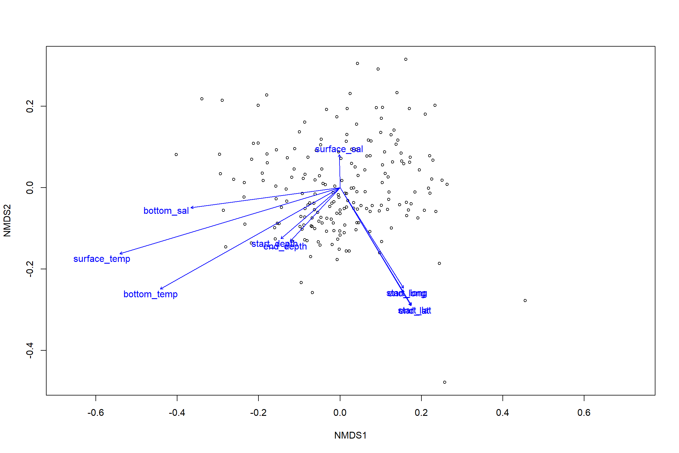
en_coord_cont = as.data.frame(scores(en, "vectors")) * ordiArrowMul(en)
en_coord_cat = as.data.frame(scores(en, "factors")) * ordiArrowMul(en)

#extract NMDS scores for ggplot
data.scores = as.data.frame(scores(nmds))
#add columns to data frame
data.scores$Region = all_Data$Region
data.scores$Year = all_Data$Year
data.scores$Season= all_Data$Season
data.scores$Year_groups= all_Data$YEAR_GROUPS
data.scores$Year_decades= all_Data$YEAR_DECADES
data.scores$Region_new=all_Data$REGION_NEW
data.scores$Region_year=all_Data$REGION_YEAR
data.scores$Season_year=all_Data$SEASON_YEAR

p<- ggplot()+
     geom_point(data = data.scores, aes(x = NMDS1, y = NMDS2, color=Year_groups, shape=Region_new), size = 4) +
  scale_color_colorblind()+
        geom_segment(data=en_coord_cont, aes(x = 0, y = 0, xend = NMDS1, yend = NMDS2), size =1.5, alpha = 0.5)+
   geom_text(data = en_coord_cont, aes(x = NMDS1, y = NMDS2), size=5,
       fontface = "bold", label = row.names(en_coord_cont))+
    theme(axis.title = element_text(size = 16, face = "bold"),
       panel.background = element_blank(), panel.border = element_rect(fill = NA),
       axis.ticks = element_blank(), axis.text = element_blank(), legend.key = element_blank(),
       legend.title = element_text(size = 16, face = "bold"),
       legend.text = element_text(size = 16))


p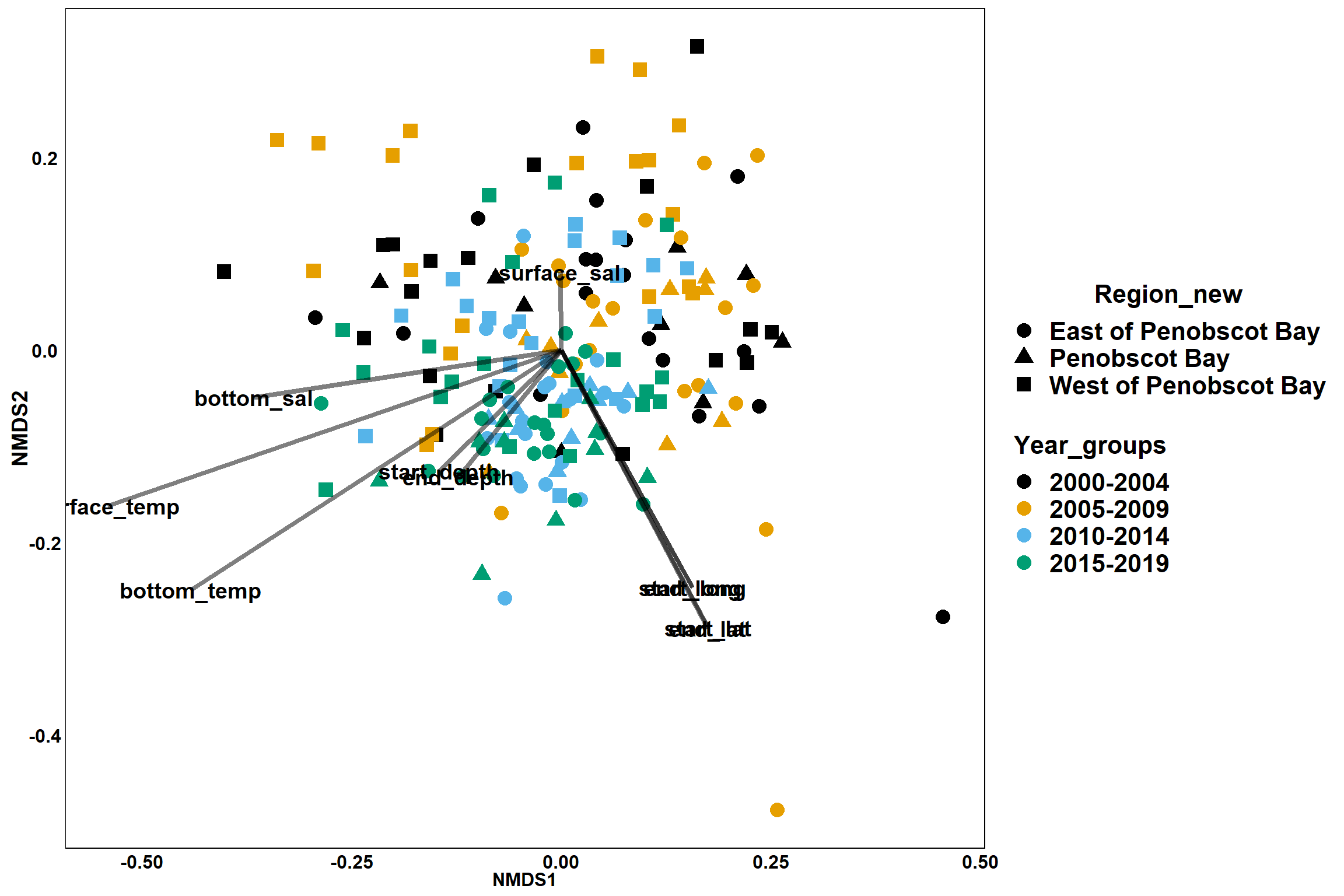
Region groups
p_region<- ggplot()+
     geom_point(data = data.scores, aes(x = NMDS1, y = NMDS2, color=Region_new), size = 4) +
  scale_color_colorblind()+
        geom_segment(data=en_coord_cont, aes(x = 0, y = 0, xend = NMDS1, yend = NMDS2), size =1.5, alpha = 0.5)+
   geom_text(data = en_coord_cont, aes(x = NMDS1, y = NMDS2), size=5,
       fontface = "bold", label = row.names(en_coord_cont))+
  stat_ellipse(data=data.scores, aes(x=NMDS1, y=NMDS2, color=Region_new),level = 0.95,size=1)+
  theme(axis.title = element_text(size = 16, face = "bold"),
       panel.background = element_blank(), panel.border = element_rect(fill = NA),
       axis.ticks = element_blank(), axis.text = element_blank(), legend.key = element_blank(),
       legend.title = element_text(size = 16, face = "bold"),
       legend.text = element_text(size = 16))


p_region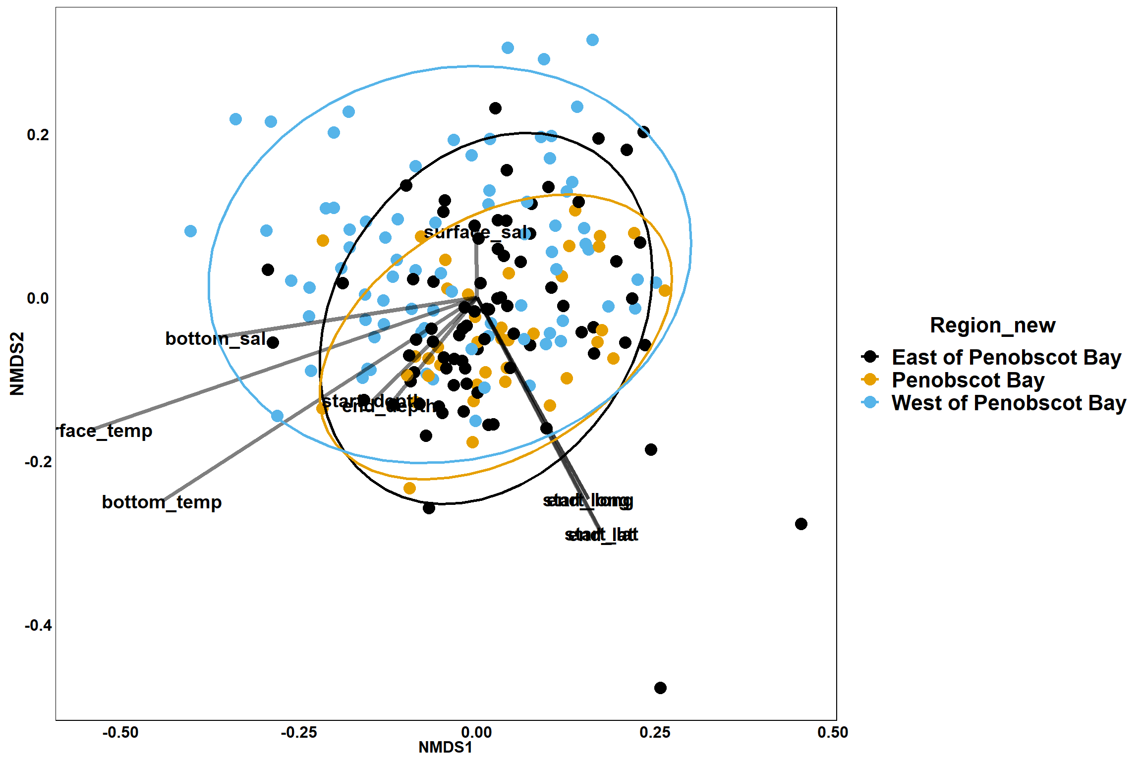
Year groups
p_year<- ggplot()+
     geom_point(data = data.scores, aes(x = NMDS1, y = NMDS2, color=Year_groups), size = 4) +
  scale_color_colorblind()+
        geom_segment(data=en_coord_cont, aes(x = 0, y = 0, xend = NMDS1, yend = NMDS2), size =1.5, alpha = 0.5)+
   geom_text(data = en_coord_cont, aes(x = NMDS1, y = NMDS2), size=5,
       fontface = "bold", label = row.names(en_coord_cont))+
  stat_ellipse(data=data.scores, aes(x=NMDS1, y=NMDS2, color=Year_groups),level = 0.95,size=1)+
  theme(axis.title = element_text(size = 16, face = "bold"),
       panel.background = element_blank(), panel.border = element_rect(fill = NA),
       axis.ticks = element_blank(), axis.text = element_blank(), legend.key = element_blank(),
       legend.title = element_text(size = 16, face = "bold"),
       legend.text = element_text(size = 16))

p_year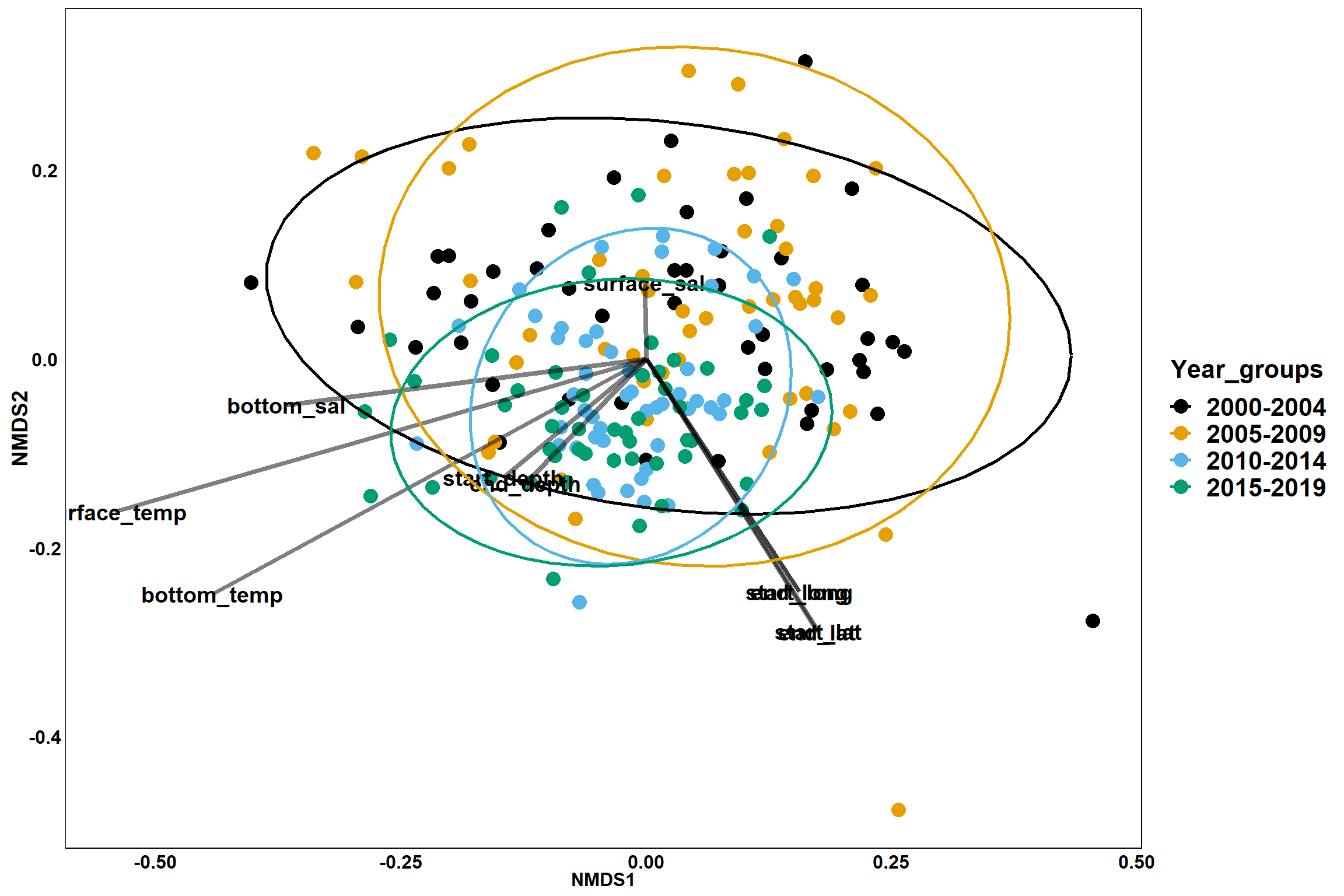
GAM contours for environmental effects
Bottom temperature
bottom_temp<-ordisurf(nmds, env$bottom_temp)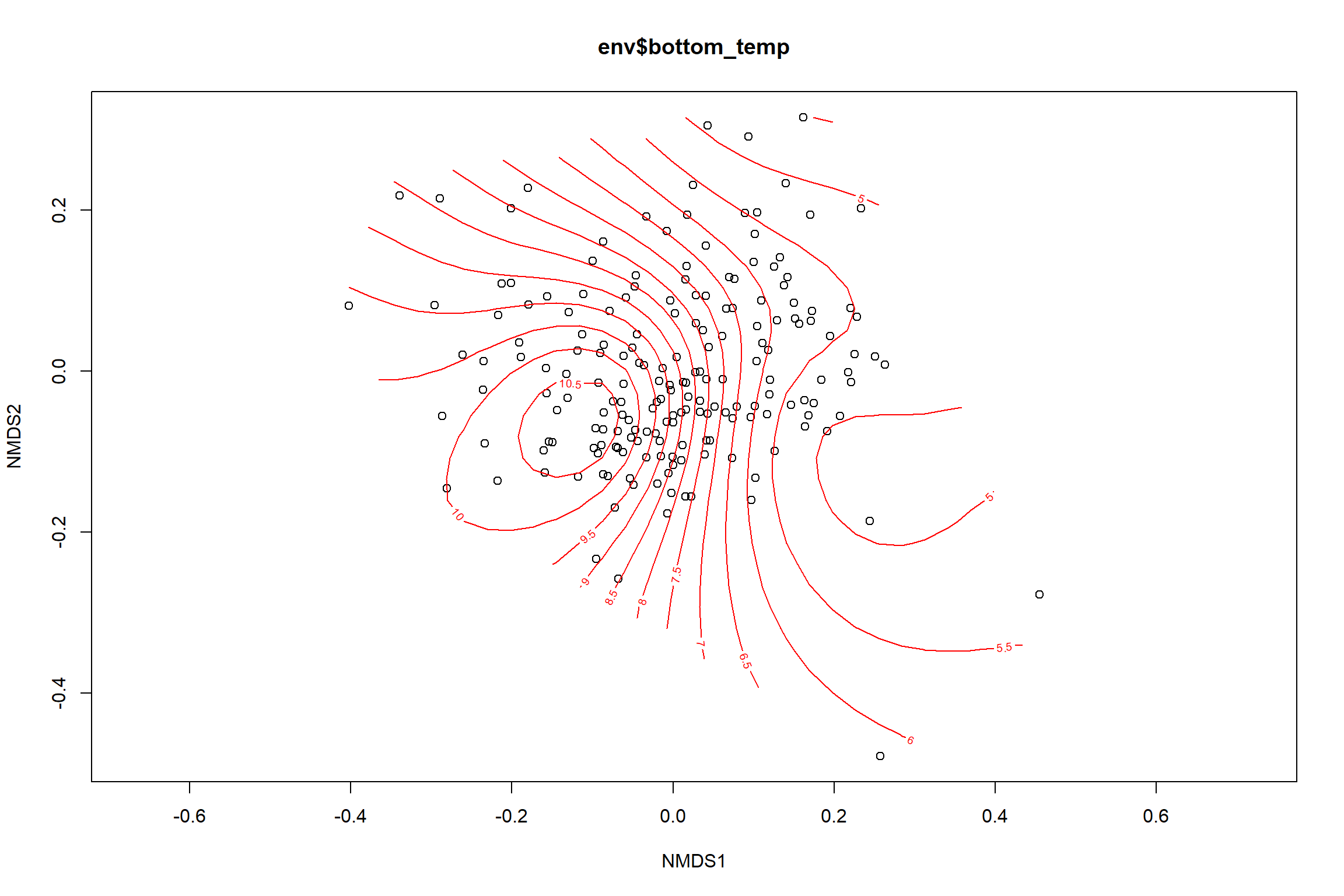
summary(bottom_temp)##
## Family: gaussian
## Link function: identity
##
## Formula:
## y ~ s(x1, x2, k = 10, bs = "tp", fx = FALSE)
##
## Parametric coefficients:
## Estimate Std. Error t value Pr(>|t|)
## (Intercept) 7.9053 0.1279 61.82 <2e-16 ***
## ---
## Signif. codes: 0 '***' 0.001 '**' 0.01 '*' 0.05 '.' 0.1 ' ' 1
##
## Approximate significance of smooth terms:
## edf Ref.df F p-value
## s(x1,x2) 7.679 9 24.65 <2e-16 ***
## ---
## Signif. codes: 0 '***' 0.001 '**' 0.01 '*' 0.05 '.' 0.1 ' ' 1
##
## R-sq.(adj) = 0.54 Deviance explained = 55.9%
## -REML = 388.52 Scale est. = 3.1069 n = 190ordi.grid <- bottom_temp$grid #extracts the ordisurf object
#str(ordi.grid) #it's a list though - cannot be plotted as is
ordi.mite <- expand.grid(x = ordi.grid$x, y = ordi.grid$y) #get x and ys
ordi.mite$z <- as.vector(ordi.grid$z) #unravel the matrix for the z scores
contour.vals <- data.frame(na.omit(ordi.mite)) #gets rid of the nas
p <- ggplot()+
stat_contour(data = contour.vals, aes(x, y, z=z, color = ..level..),position="identity",size=1.5)+
labs(x = "NMDS1", y = "NMDS2", color="Bottom Temperature")+
new_scale_color()+
geom_point(data = data.scores, aes(NMDS1, NMDS2, color=Year_groups, shape=Region_new), size = 3 )+ scale_color_colorblind()
p1 <- ggplot()+
stat_contour(data = contour.vals, aes(x, y, z=z, color = ..level..),position="identity",size=1.5)+
labs(x = "NMDS1", y = "NMDS2", color="Bottom Temperature")+
new_scale_color()+
geom_point(data = data.scores, aes(NMDS1, NMDS2, color=Year_groups), size = 2 )+ stat_ellipse(data=data.scores, aes(x=NMDS1, y=NMDS2, color=Year_groups),level = 0.95,size=1)+
scale_color_colorblind()
p2 <- ggplot()+
stat_contour(data = contour.vals, aes(x, y, z=z, color = ..level..),position="identity",size=1.5)+
labs(x = "NMDS1", y = "NMDS2", color="Bottom Temperature")+
new_scale_color()+
geom_point(data = data.scores, aes(NMDS1, NMDS2, color=Region_new), size = 2 )+
stat_ellipse(data=data.scores, aes(x=NMDS1, y=NMDS2, color=Region_new),level = 0.95,size=1)+
scale_color_colorblind()
p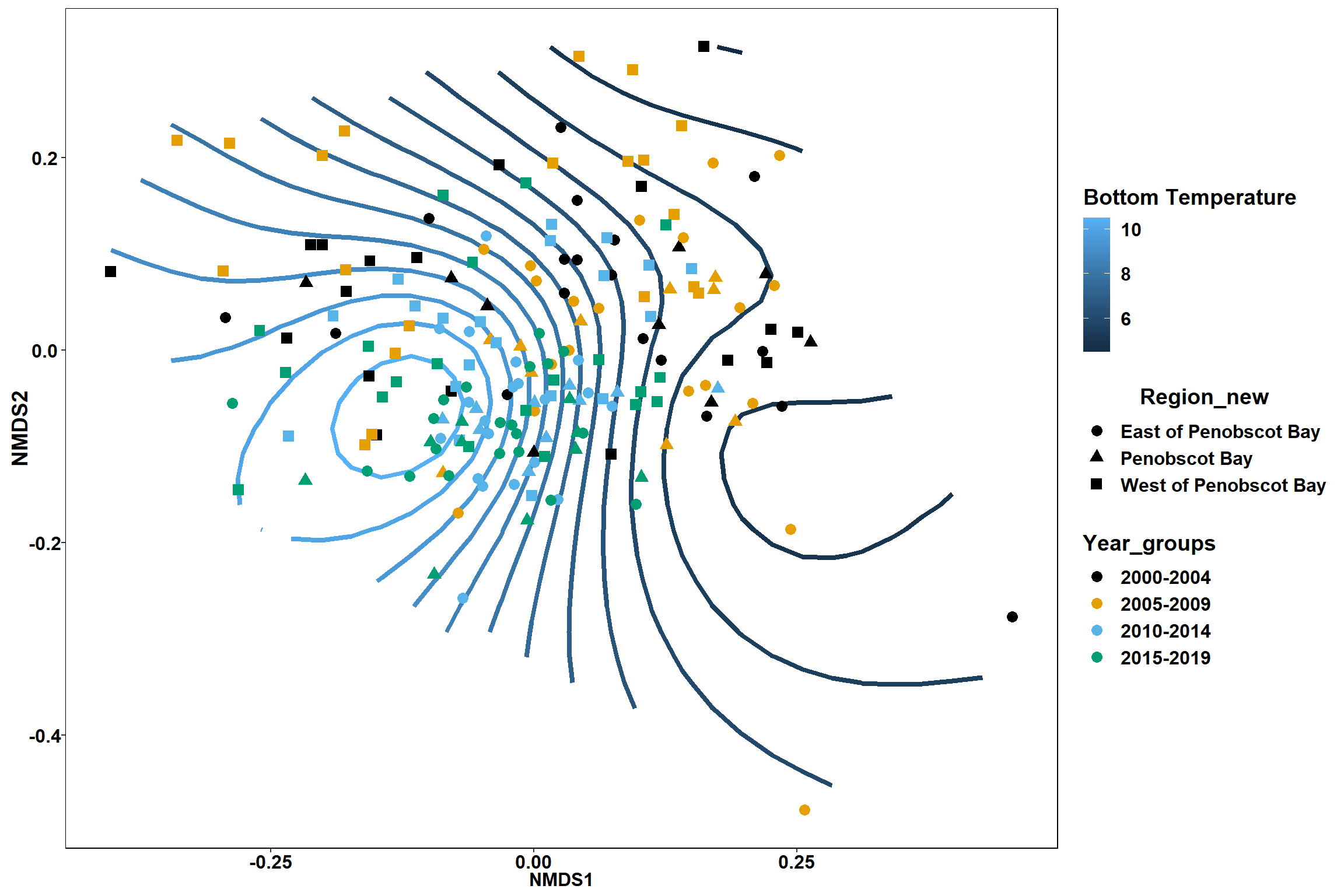
p1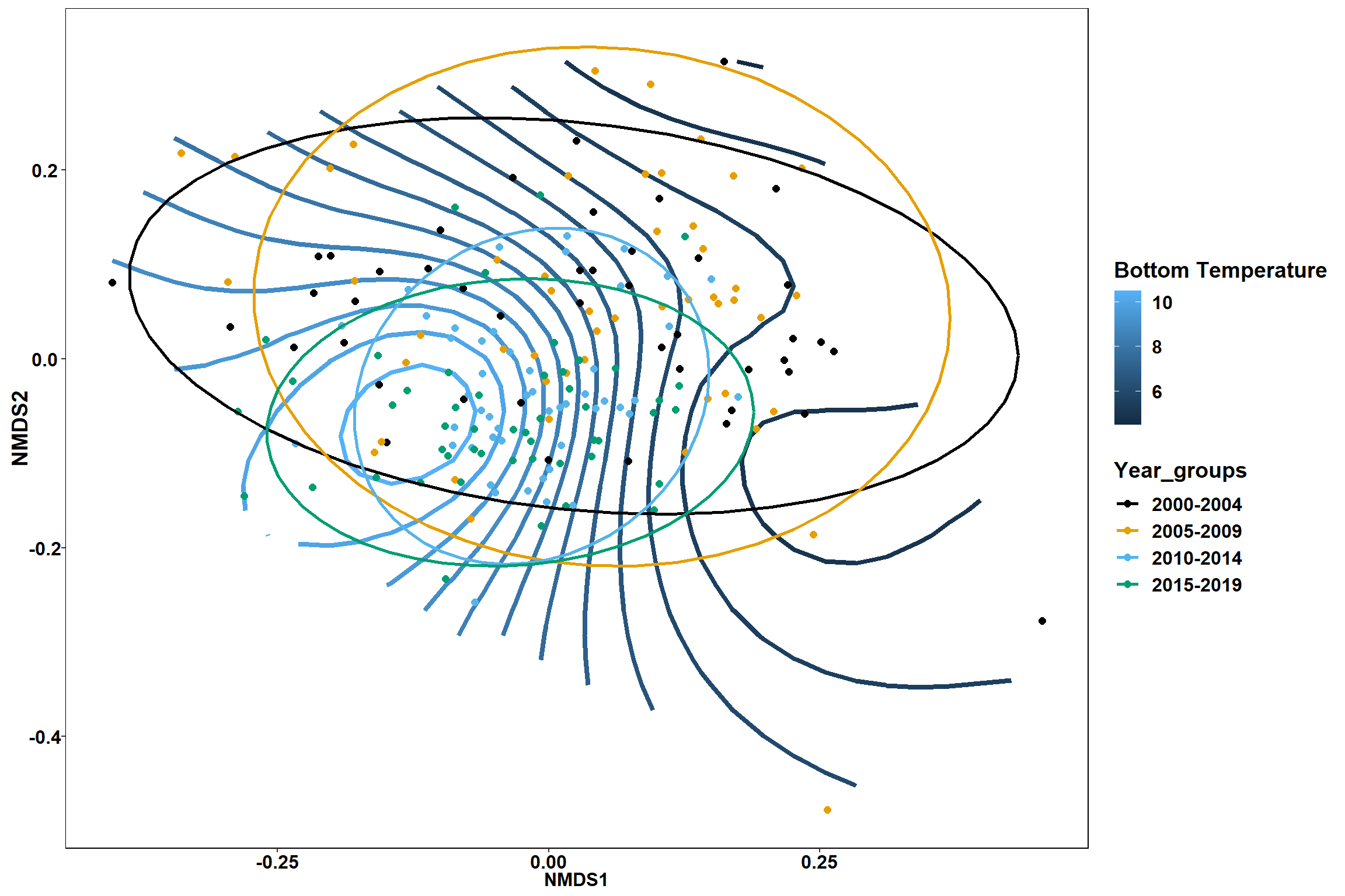
p2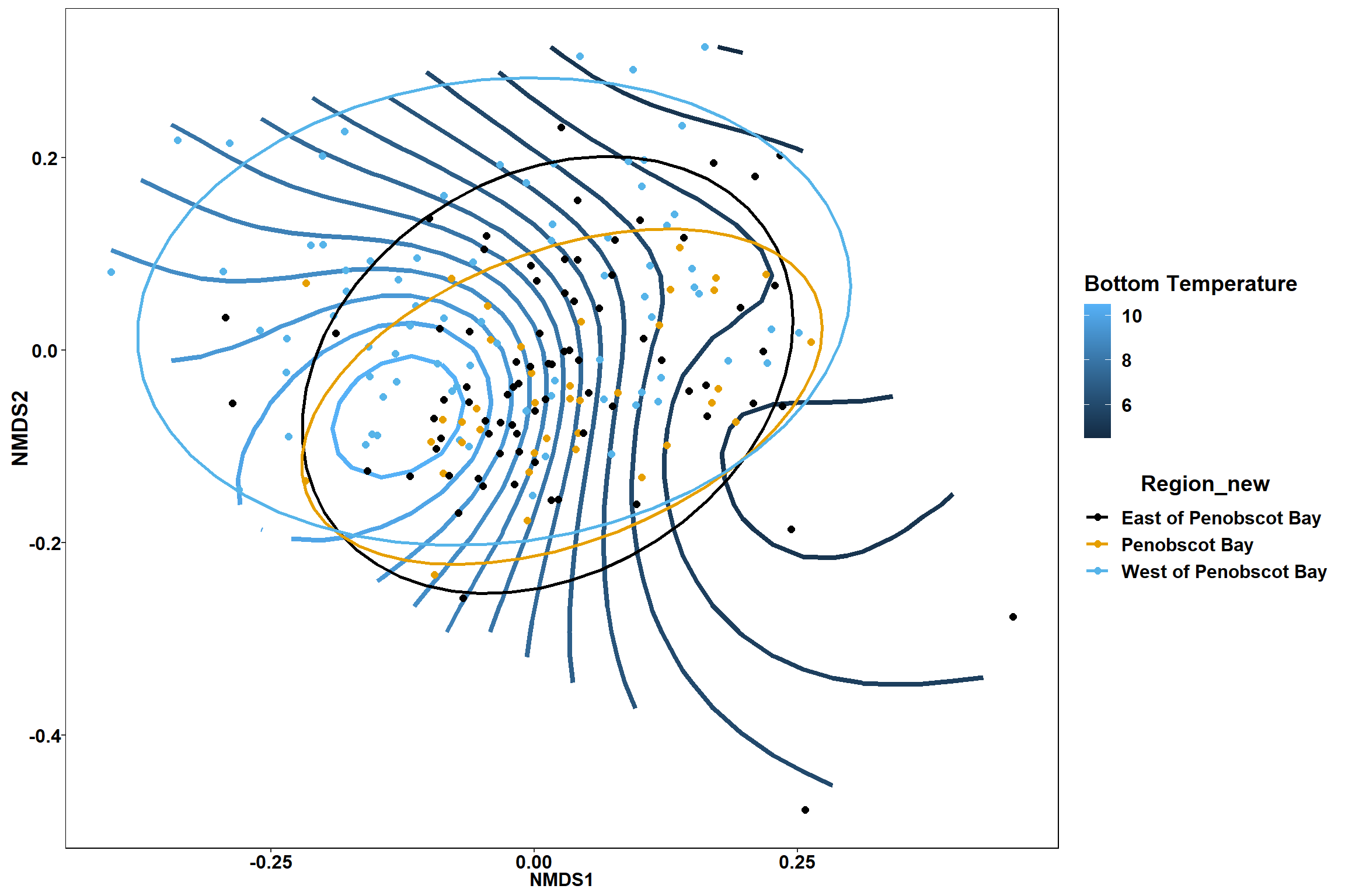
Surface temperature
surface_temp<-ordisurf(nmds, env$surface_temp)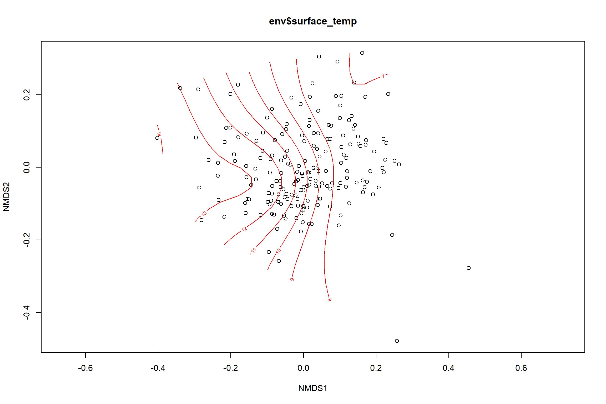
summary(surface_temp)##
## Family: gaussian
## Link function: identity
##
## Formula:
## y ~ s(x1, x2, k = 10, bs = "tp", fx = FALSE)
##
## Parametric coefficients:
## Estimate Std. Error t value Pr(>|t|)
## (Intercept) 9.770 0.125 78.17 <2e-16 ***
## ---
## Signif. codes: 0 '***' 0.001 '**' 0.01 '*' 0.05 '.' 0.1 ' ' 1
##
## Approximate significance of smooth terms:
## edf Ref.df F p-value
## s(x1,x2) 7.801 9 31.48 <2e-16 ***
## ---
## Signif. codes: 0 '***' 0.001 '**' 0.01 '*' 0.05 '.' 0.1 ' ' 1
##
## R-sq.(adj) = 0.6 Deviance explained = 61.6%
## -REML = 384.57 Scale est. = 2.9679 n = 190ordi.grid <- surface_temp$grid #extracts the ordisurf object
#str(ordi.grid) #it's a list though - cannot be plotted as is
ordi.mite <- expand.grid(x = ordi.grid$x, y = ordi.grid$y) #get x and ys
ordi.mite$z <- as.vector(ordi.grid$z) #unravel the matrix for the z scores
contour.vals <- data.frame(na.omit(ordi.mite)) #gets rid of the nas
p <- ggplot()+
stat_contour(data = contour.vals, aes(x, y, z=z, color = ..level..),position="identity",size=1.5)+
labs(x = "NMDS1", y = "NMDS2", color="Surface Temperature")+
new_scale_color()+
geom_point(data = data.scores, aes(NMDS1, NMDS2, color=Year_groups, shape=Region_new), size = 3 )+ scale_color_colorblind()
p1 <- ggplot()+
stat_contour(data = contour.vals, aes(x, y, z=z, color = ..level..),position="identity",size=1.5)+
labs(x = "NMDS1", y = "NMDS2", color="Surface Temperature")+
new_scale_color()+
geom_point(data = data.scores, aes(NMDS1, NMDS2, color=Year_groups), size = 2 )+stat_ellipse(data=data.scores, aes(x=NMDS1, y=NMDS2, color=Year_groups),level = 0.95,size=1)+
scale_color_colorblind()
p2 <- ggplot()+
stat_contour(data = contour.vals, aes(x, y, z=z, color = ..level..),position="identity",size=1.5)+
labs(x = "NMDS1", y = "NMDS2", color="Surface Temperature")+
new_scale_color()+
geom_point(data = data.scores, aes(NMDS1, NMDS2, color=Region_new), size = 2 )+stat_ellipse(data=data.scores, aes(x=NMDS1, y=NMDS2, color=Region_new),level = 0.95,size=1)+
scale_color_colorblind()
p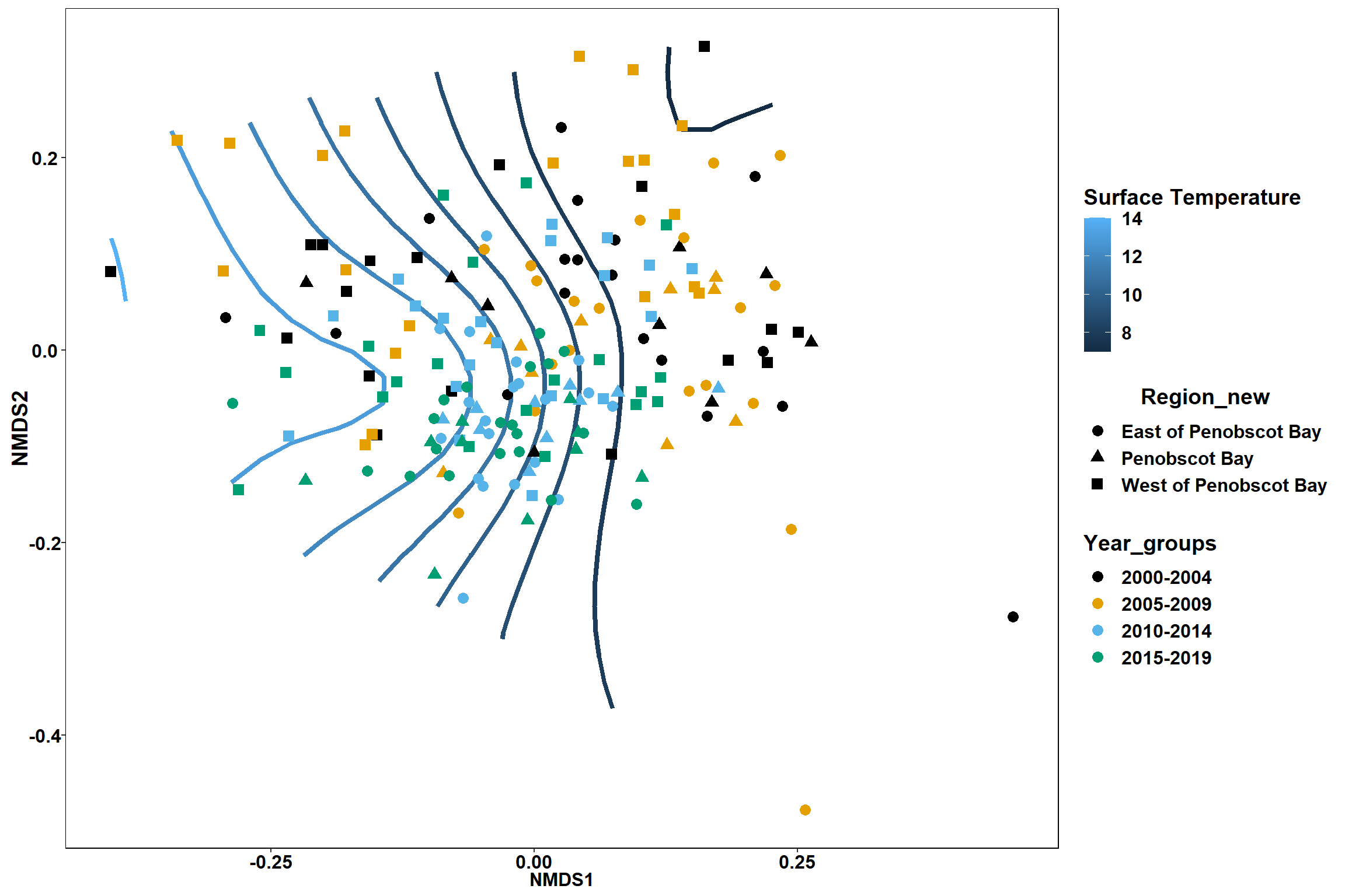
p1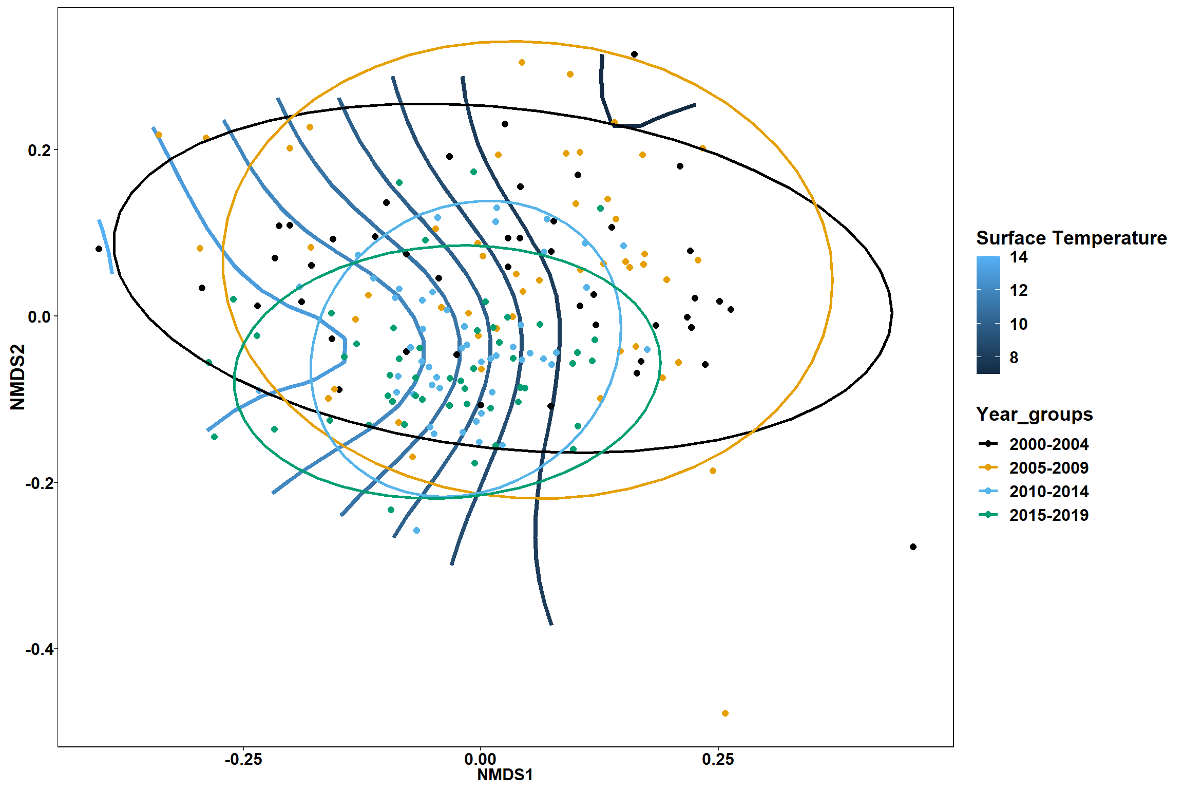
p2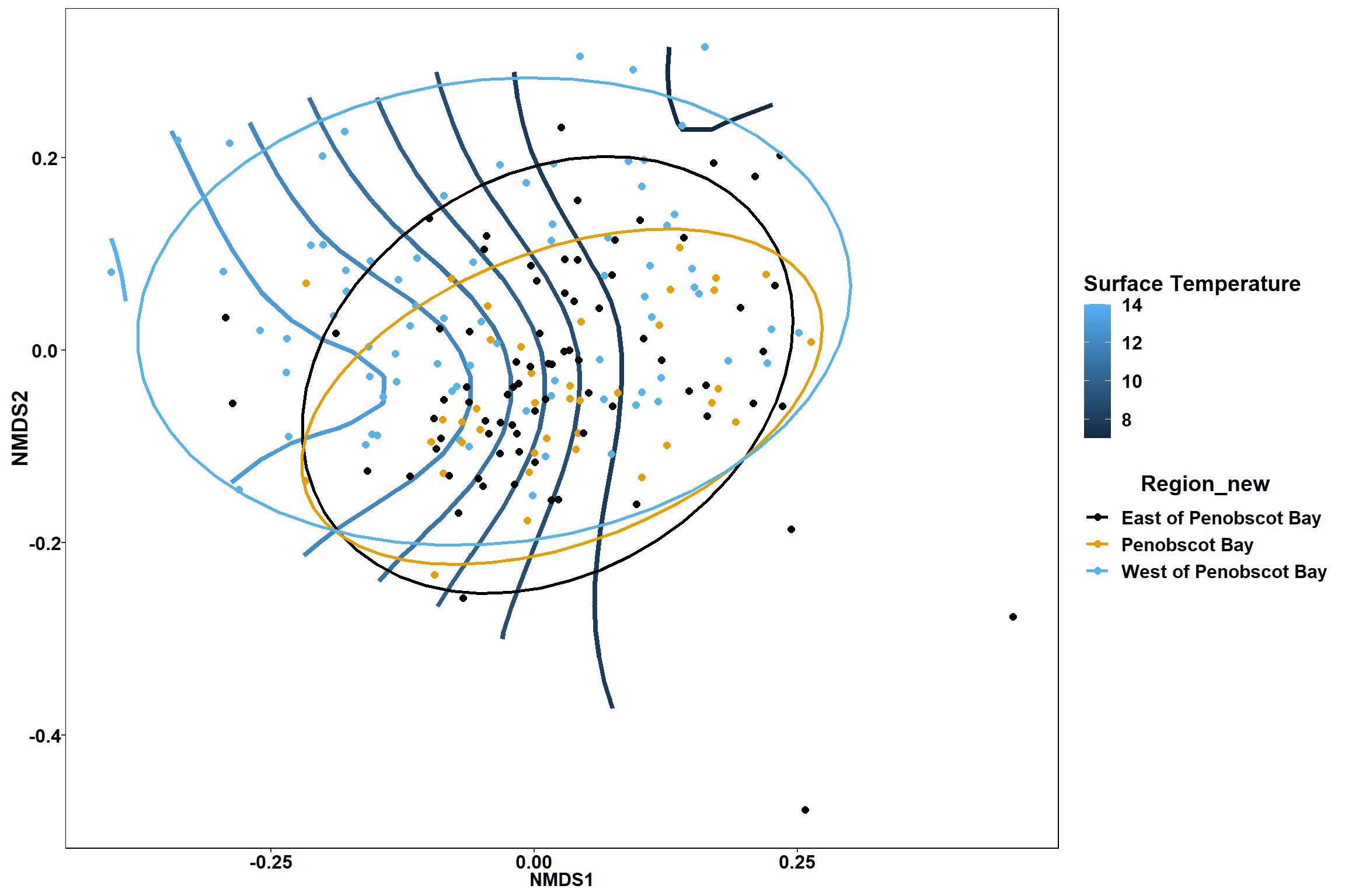
Bottom salinity
bottom_sal<-ordisurf(nmds, env$bottom_sal)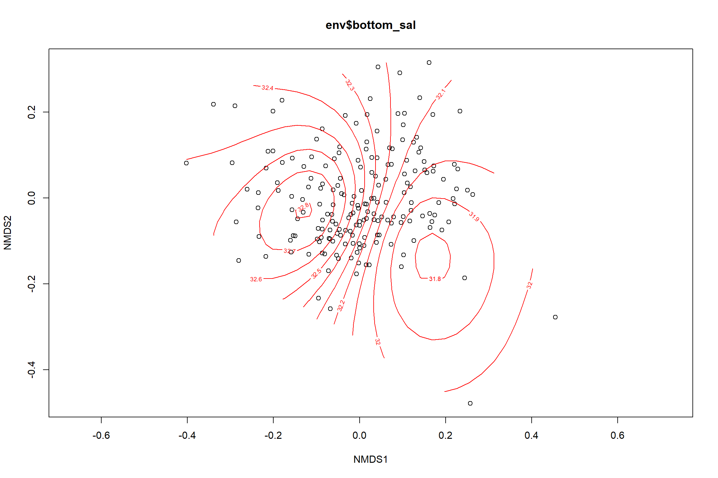
summary(bottom_sal)##
## Family: gaussian
## Link function: identity
##
## Formula:
## y ~ s(x1, x2, k = 10, bs = "tp", fx = FALSE)
##
## Parametric coefficients:
## Estimate Std. Error t value Pr(>|t|)
## (Intercept) 32.33134 0.03023 1069 <2e-16 ***
## ---
## Signif. codes: 0 '***' 0.001 '**' 0.01 '*' 0.05 '.' 0.1 ' ' 1
##
## Approximate significance of smooth terms:
## edf Ref.df F p-value
## s(x1,x2) 6.248 9 10.92 <2e-16 ***
## ---
## Signif. codes: 0 '***' 0.001 '**' 0.01 '*' 0.05 '.' 0.1 ' ' 1
##
## R-sq.(adj) = 0.342 Deviance explained = 36.4%
## -REML = 113.14 Scale est. = 0.17365 n = 190ordi.grid <- bottom_sal$grid #extracts the ordisurf object
#str(ordi.grid) #it's a list though - cannot be plotted as is
ordi.mite <- expand.grid(x = ordi.grid$x, y = ordi.grid$y) #get x and ys
ordi.mite$z <- as.vector(ordi.grid$z) #unravel the matrix for the z scores
contour.vals <- data.frame(na.omit(ordi.mite)) #gets rid of the nas
p <- ggplot()+
stat_contour(data = contour.vals, aes(x, y, z=z, color = ..level..),position="identity",size=1.5)+
labs(x = "NMDS1", y = "NMDS2", color="Bottom Salinity")+
new_scale_color()+
geom_point(data = data.scores, aes(NMDS1, NMDS2, color=Year_groups, shape=Region_new), size = 3 )+ scale_color_colorblind()
p1 <- ggplot()+
stat_contour(data = contour.vals, aes(x, y, z=z, color = ..level..),position="identity",size=1.5)+
labs(x = "NMDS1", y = "NMDS2", color="Bottom Salinity")+
new_scale_color()+
geom_point(data = data.scores, aes(NMDS1, NMDS2, color=Year_groups), size = 2 )+ stat_ellipse(data=data.scores, aes(x=NMDS1, y=NMDS2, color=Year_groups),level = 0.95,size=1)+
scale_color_colorblind()
p2 <- ggplot()+
stat_contour(data = contour.vals, aes(x, y, z=z, color = ..level..),position="identity",size=1.5)+
labs(x = "NMDS1", y = "NMDS2", color="Bottom Salinity")+
new_scale_color()+
geom_point(data = data.scores, aes(NMDS1, NMDS2, color=Region_new), size = 2 )+stat_ellipse(data=data.scores, aes(x=NMDS1, y=NMDS2, color=Region_new),level = 0.95,size=1)+
scale_color_colorblind()
p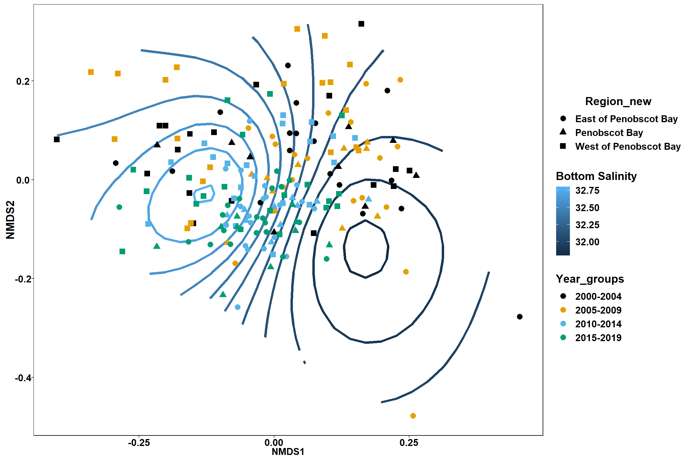
p1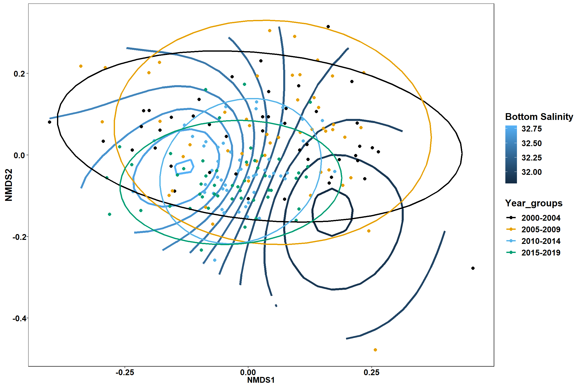
p2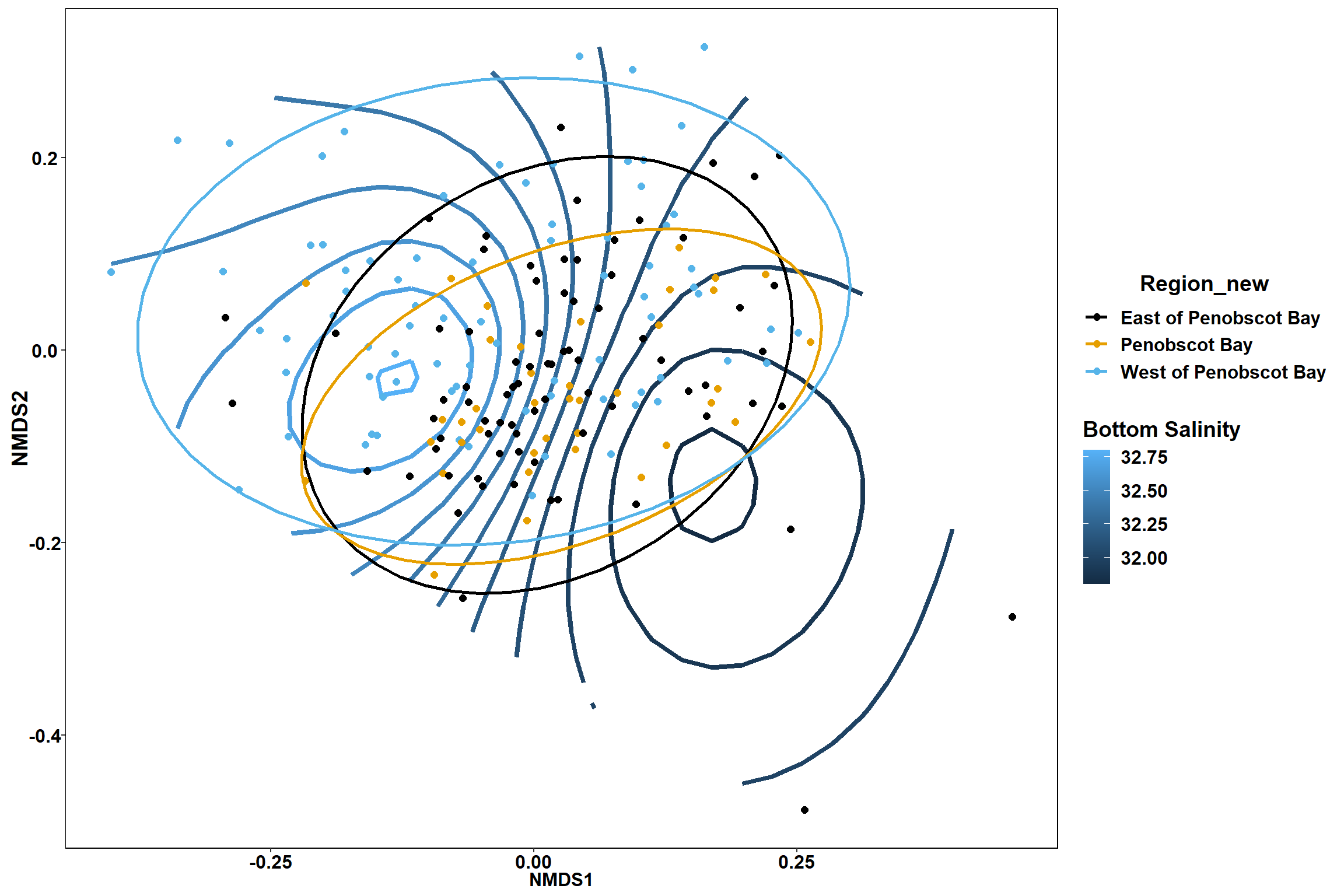
Surface salinity
surface_sal<-ordisurf(nmds, env$surface_sal)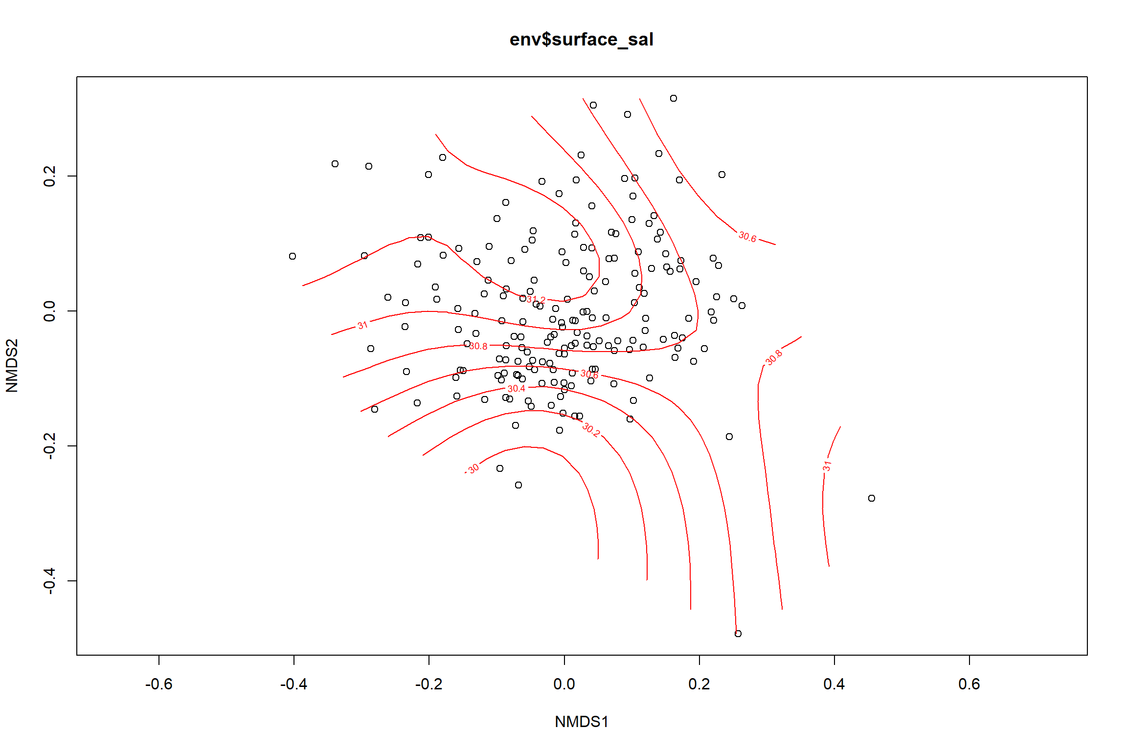
summary(surface_sal)##
## Family: gaussian
## Link function: identity
##
## Formula:
## y ~ s(x1, x2, k = 10, bs = "tp", fx = FALSE)
##
## Parametric coefficients:
## Estimate Std. Error t value Pr(>|t|)
## (Intercept) 30.8492 0.2316 133.2 <2e-16 ***
## ---
## Signif. codes: 0 '***' 0.001 '**' 0.01 '*' 0.05 '.' 0.1 ' ' 1
##
## Approximate significance of smooth terms:
## edf Ref.df F p-value
## s(x1,x2) 2.579 9 0.482 0.13
##
## R-sq.(adj) = 0.0224 Deviance explained = 3.58%
## -REML = 491.96 Scale est. = 10.191 n = 190ordi.grid <- surface_sal$grid #extracts the ordisurf object
#str(ordi.grid) #it's a list though - cannot be plotted as is
ordi.mite <- expand.grid(x = ordi.grid$x, y = ordi.grid$y) #get x and ys
ordi.mite$z <- as.vector(ordi.grid$z) #unravel the matrix for the z scores
contour.vals <- data.frame(na.omit(ordi.mite)) #gets rid of the nas
p <- ggplot()+
stat_contour(data = contour.vals, aes(x, y, z=z, color = ..level..),position="identity",size=1.5)+
labs(x = "NMDS1", y = "NMDS2", color="Surface Salinity")+
new_scale_color()+
geom_point(data = data.scores, aes(NMDS1, NMDS2, color=Year_groups, shape=Region_new), size = 3 )+ scale_color_colorblind()
p1 <- ggplot()+
stat_contour(data = contour.vals, aes(x, y, z=z, color = ..level..),position="identity",size=1.5)+
labs(x = "NMDS1", y = "NMDS2", color="Surface Salinity")+
new_scale_color()+
geom_point(data = data.scores, aes(NMDS1, NMDS2, color=Year_groups), size = 2 )+stat_ellipse(data=data.scores, aes(x=NMDS1, y=NMDS2, color=Year_groups),level = 0.95,size=1)+
scale_color_colorblind()
p2 <- ggplot()+
stat_contour(data = contour.vals, aes(x, y, z=z, color = ..level..),position="identity",size=1.5)+
labs(x = "NMDS1", y = "NMDS2", color="Surface Salinity")+
new_scale_color()+
geom_point(data = data.scores, aes(NMDS1, NMDS2, color=Region_new), size = 2 )+stat_ellipse(data=data.scores, aes(x=NMDS1, y=NMDS2, color=Region_new),level = 0.95,size=1)+
scale_color_colorblind()
p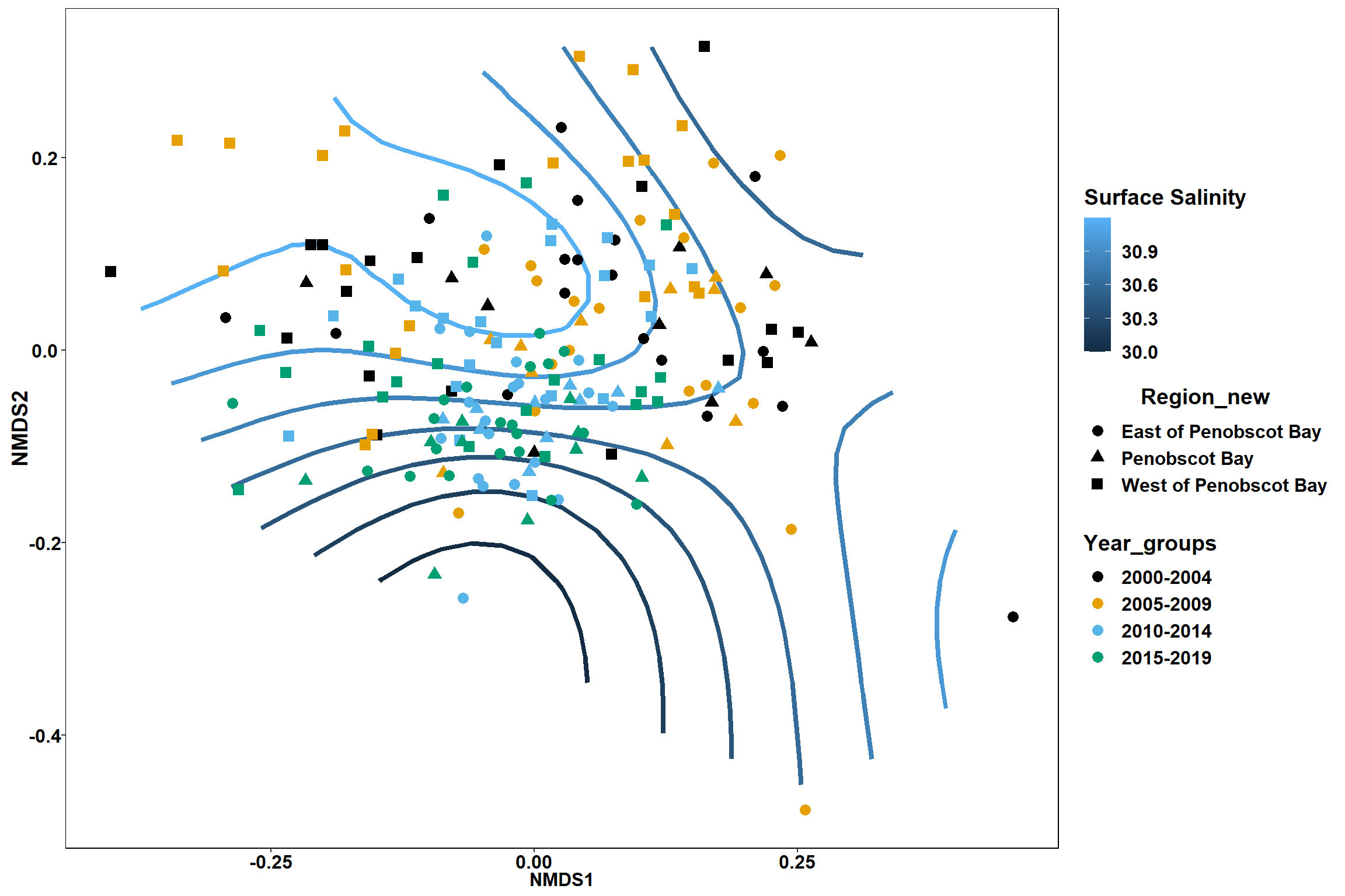
p1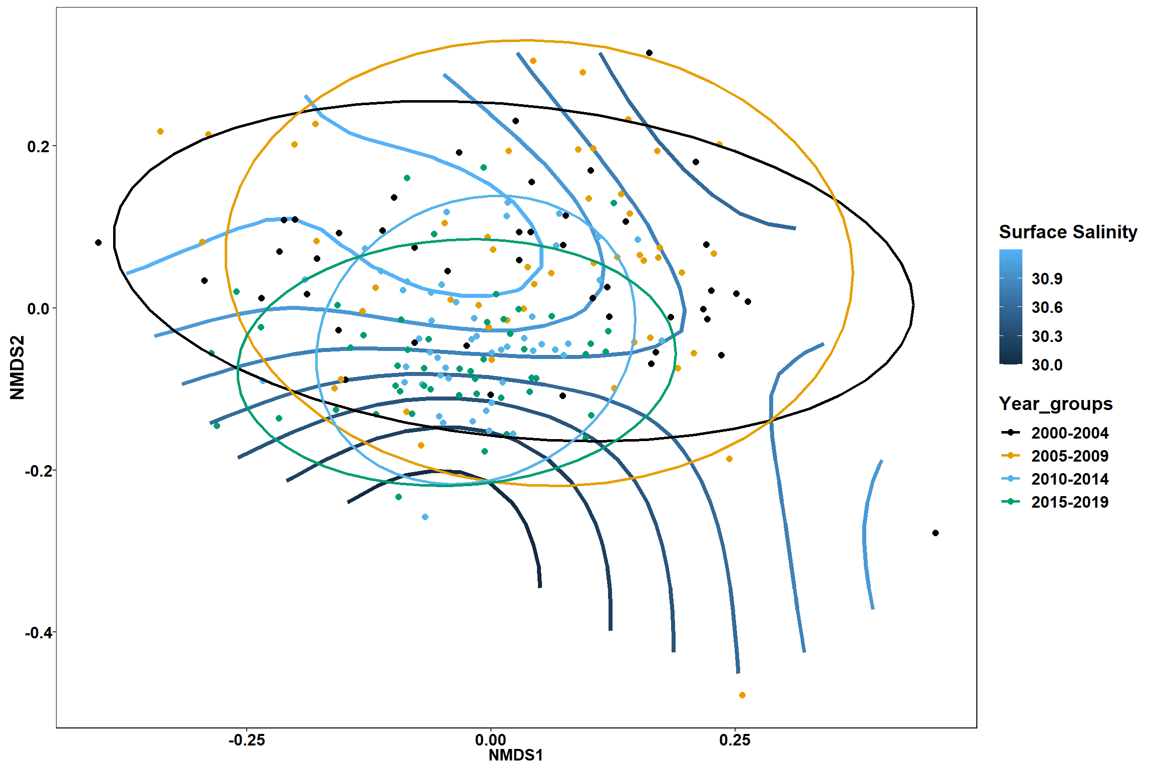
p2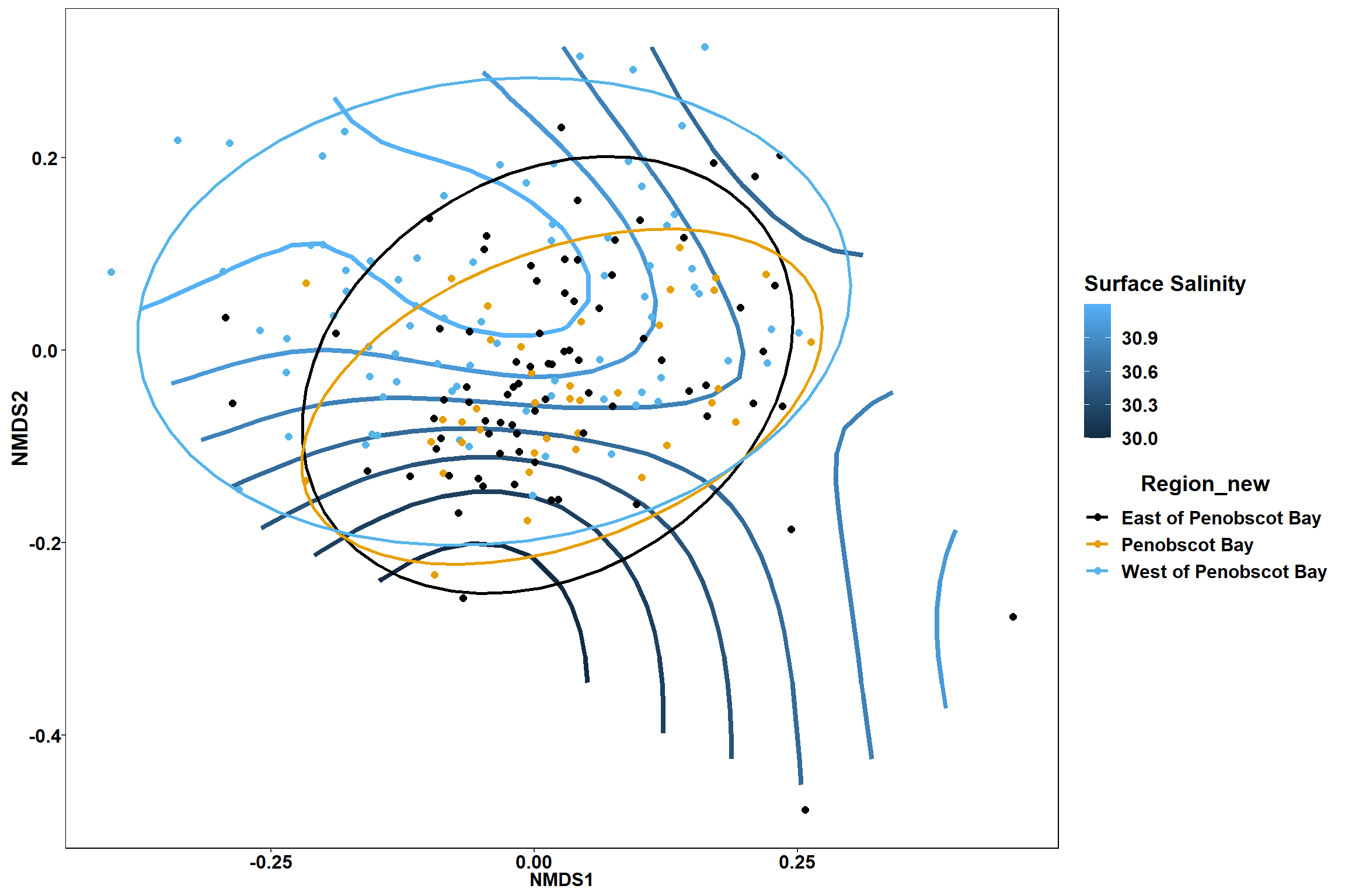
start latitude
start_lat<-ordisurf(nmds, env$start_lat)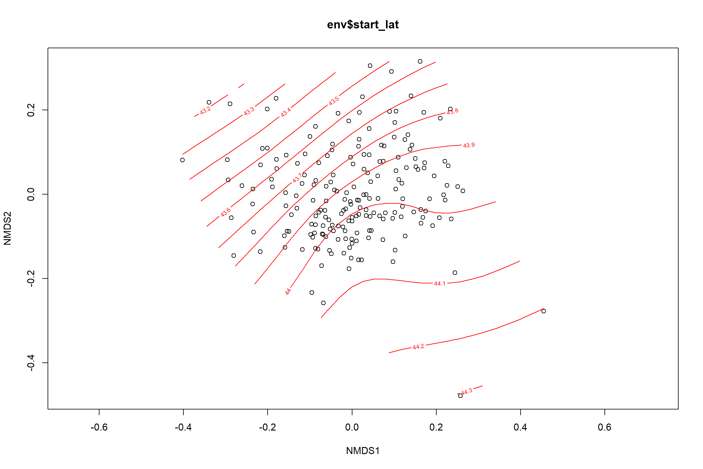
summary(start_lat)##
## Family: gaussian
## Link function: identity
##
## Formula:
## y ~ s(x1, x2, k = 10, bs = "tp", fx = FALSE)
##
## Parametric coefficients:
## Estimate Std. Error t value Pr(>|t|)
## (Intercept) 43.87499 0.02754 1593 <2e-16 ***
## ---
## Signif. codes: 0 '***' 0.001 '**' 0.01 '*' 0.05 '.' 0.1 ' ' 1
##
## Approximate significance of smooth terms:
## edf Ref.df F p-value
## s(x1,x2) 4.889 9 5.629 <2e-16 ***
## ---
## Signif. codes: 0 '***' 0.001 '**' 0.01 '*' 0.05 '.' 0.1 ' ' 1
##
## R-sq.(adj) = 0.207 Deviance explained = 22.7%
## -REML = 97.67 Scale est. = 0.14795 n = 195ordi.grid <- start_lat$grid #extracts the ordisurf object
#str(ordi.grid) #it's a list though - cannot be plotted as is
ordi.mite <- expand.grid(x = ordi.grid$x, y = ordi.grid$y) #get x and ys
ordi.mite$z <- as.vector(ordi.grid$z) #unravel the matrix for the z scores
contour.vals <- data.frame(na.omit(ordi.mite)) #gets rid of the nas
p <- ggplot()+
stat_contour(data = contour.vals, aes(x, y, z=z, color = ..level..),position="identity",size=1.5)+
labs(x = "NMDS1", y = "NMDS2", color="Latitude")+
new_scale_color()+
geom_point(data = data.scores, aes(NMDS1, NMDS2, color=Year_groups, shape=Region_new), size = 3 )+ scale_color_colorblind()
p1 <- ggplot()+
stat_contour(data = contour.vals, aes(x, y, z=z, color = ..level..),position="identity",size=1.5)+
labs(x = "NMDS1", y = "NMDS2", color="Latitude")+
new_scale_color()+
geom_point(data = data.scores, aes(NMDS1, NMDS2, color=Year_groups), size = 2 )+ stat_ellipse(data=data.scores, aes(x=NMDS1, y=NMDS2, color=Year_groups),level = 0.95,size=1)+
scale_color_colorblind()
p2 <- ggplot()+
stat_contour(data = contour.vals, aes(x, y, z=z, color = ..level..),position="identity",size=1.5)+
labs(x = "NMDS1", y = "NMDS2", color="Latitude")+
new_scale_color()+
geom_point(data = data.scores, aes(NMDS1, NMDS2, color=Region_new), size = 2 )+ stat_ellipse(data=data.scores, aes(x=NMDS1, y=NMDS2, color=Region_new),level = 0.95,size=1)+
scale_color_colorblind()
p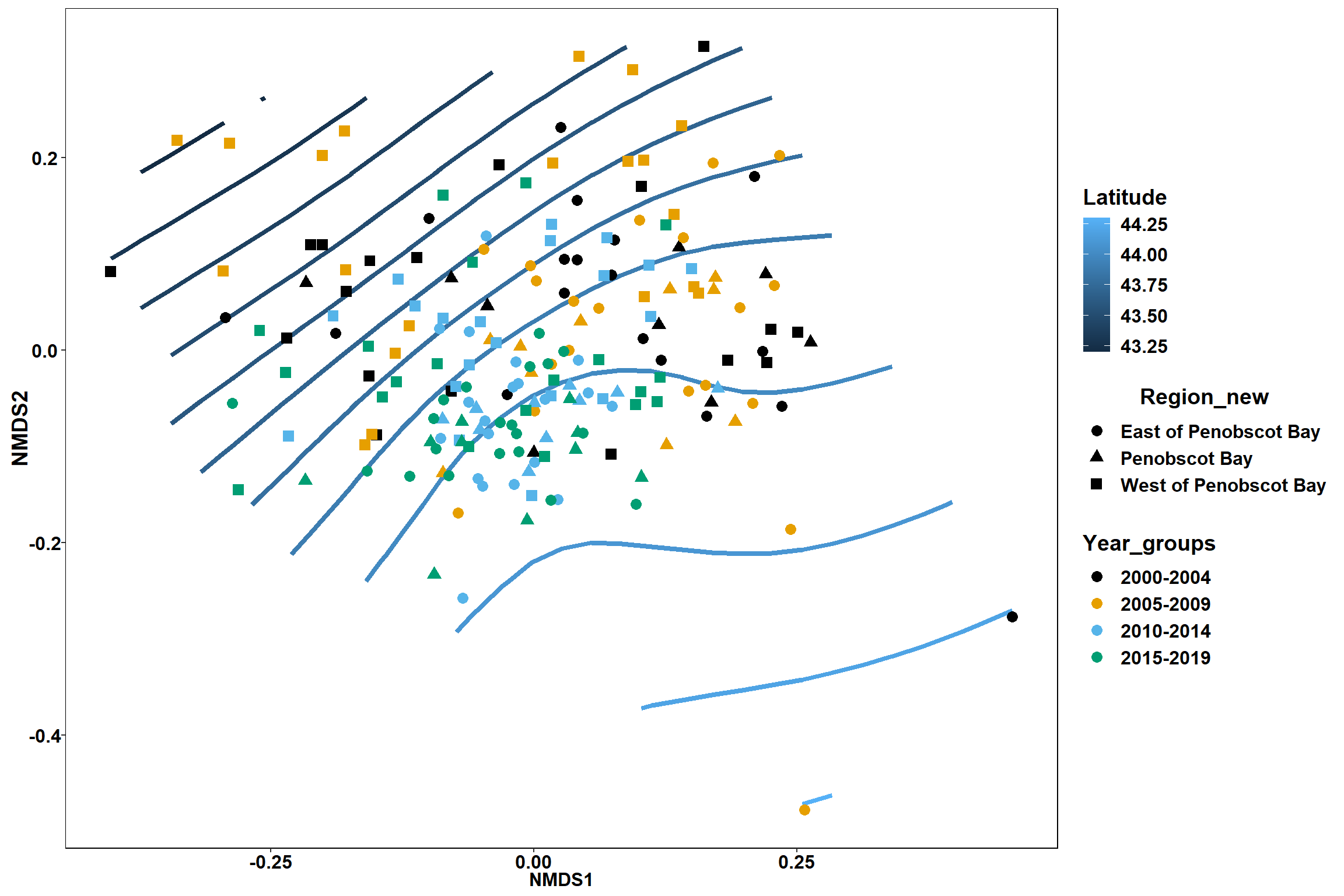
p1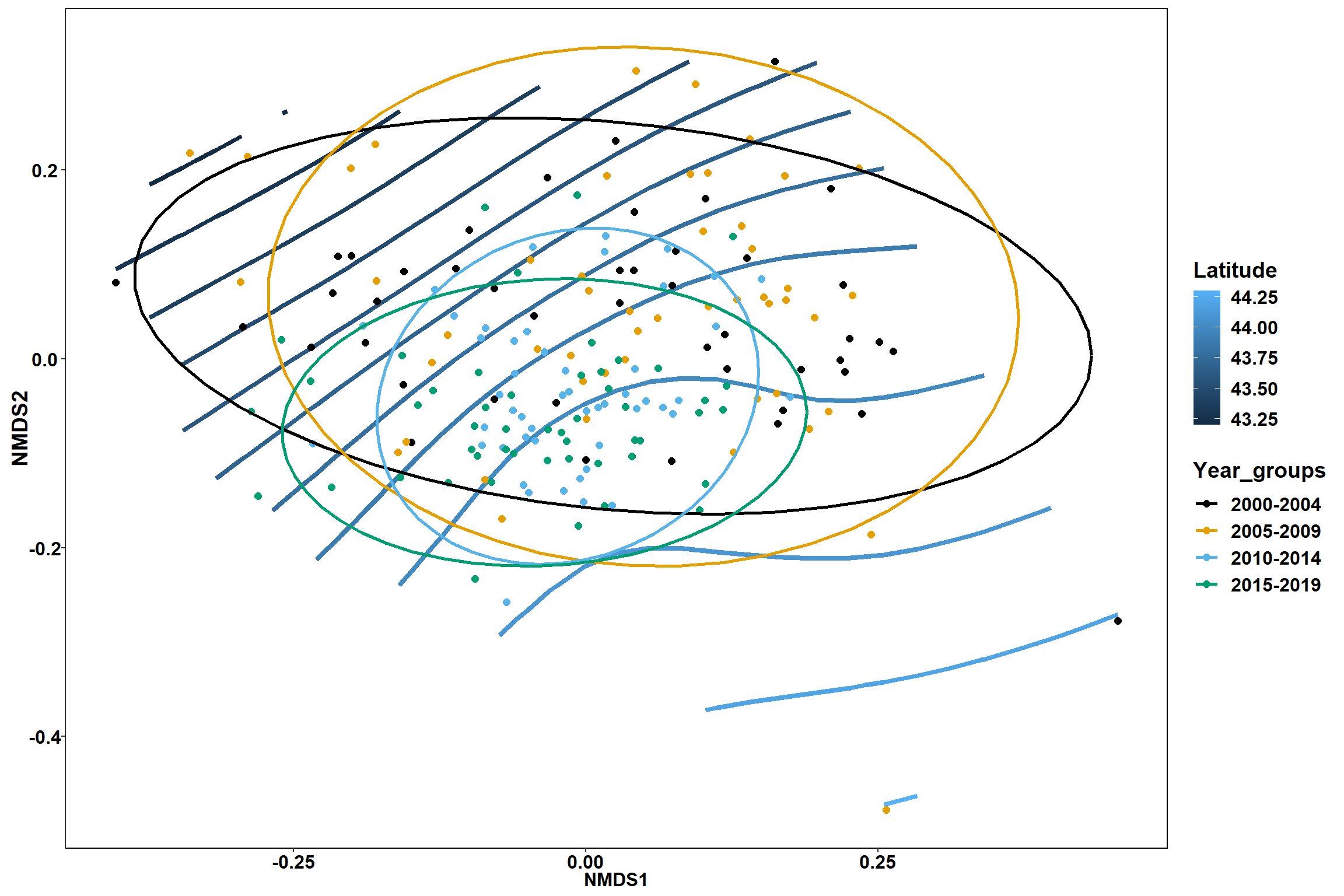
p2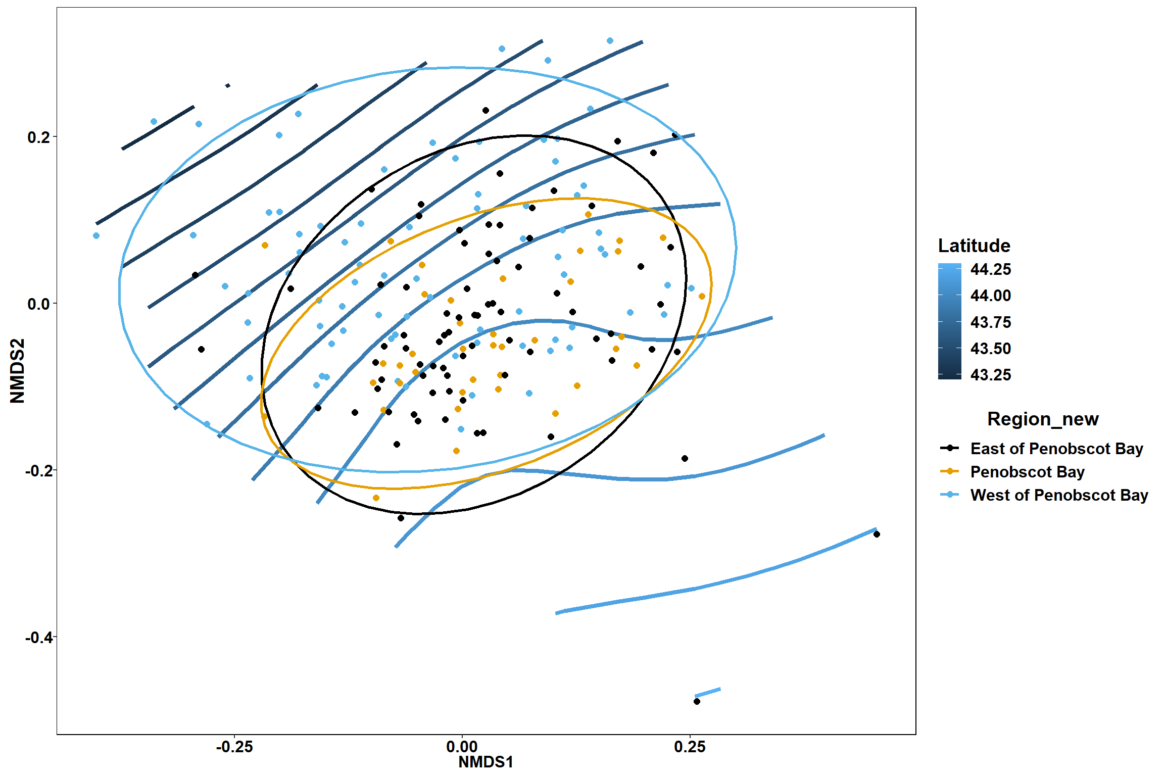
start longitude
start_long<-ordisurf(nmds, env$start_long)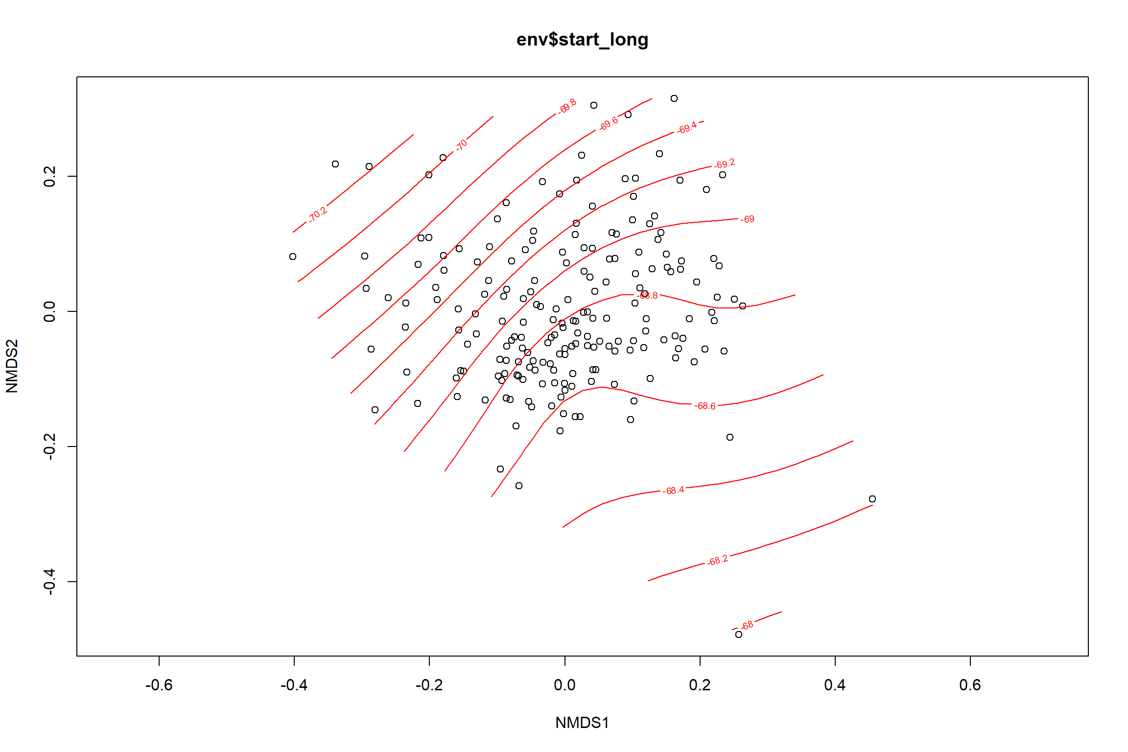
summary(start_long)##
## Family: gaussian
## Link function: identity
##
## Formula:
## y ~ s(x1, x2, k = 10, bs = "tp", fx = FALSE)
##
## Parametric coefficients:
## Estimate Std. Error t value Pr(>|t|)
## (Intercept) -68.97337 0.06801 -1014 <2e-16 ***
## ---
## Signif. codes: 0 '***' 0.001 '**' 0.01 '*' 0.05 '.' 0.1 ' ' 1
##
## Approximate significance of smooth terms:
## edf Ref.df F p-value
## s(x1,x2) 4.332 9 3.746 7.49e-07 ***
## ---
## Signif. codes: 0 '***' 0.001 '**' 0.01 '*' 0.05 '.' 0.1 ' ' 1
##
## R-sq.(adj) = 0.148 Deviance explained = 16.7%
## -REML = 272.24 Scale est. = 0.90208 n = 195ordi.grid <- start_long$grid #extracts the ordisurf object
#str(ordi.grid) #it's a list though - cannot be plotted as is
ordi.mite <- expand.grid(x = ordi.grid$x, y = ordi.grid$y) #get x and ys
ordi.mite$z <- as.vector(ordi.grid$z) #unravel the matrix for the z scores
contour.vals <- data.frame(na.omit(ordi.mite)) #gets rid of the nas
p <- ggplot()+
stat_contour(data = contour.vals, aes(x, y, z=z, color = ..level..),position="identity",size=1.5)+
labs(x = "NMDS1", y = "NMDS2", color="Longitude")+
new_scale_color()+
geom_point(data = data.scores, aes(NMDS1, NMDS2, color=Year_groups, shape=Region_new), size = 3 )+ scale_color_colorblind()
p1 <- ggplot()+
stat_contour(data = contour.vals, aes(x, y, z=z, color = ..level..),position="identity",size=1.5)+
labs(x = "NMDS1", y = "NMDS2", color="Longitude")+
new_scale_color()+
geom_point(data = data.scores, aes(NMDS1, NMDS2, color=Year_groups), size = 2 )+stat_ellipse(data=data.scores, aes(x=NMDS1, y=NMDS2, color=Year_groups),level = 0.95,size=1)+
scale_color_colorblind()
p2 <- ggplot()+
stat_contour(data = contour.vals, aes(x, y, z=z, color = ..level..),position="identity",size=1.5)+
labs(x = "NMDS1", y = "NMDS2", color="Longitude")+
new_scale_color()+
geom_point(data = data.scores, aes(NMDS1, NMDS2, color=Region_new), size = 2 )+stat_ellipse(data=data.scores, aes(x=NMDS1, y=NMDS2, color=Region_new),level = 0.95,size=1)+
scale_color_colorblind()
p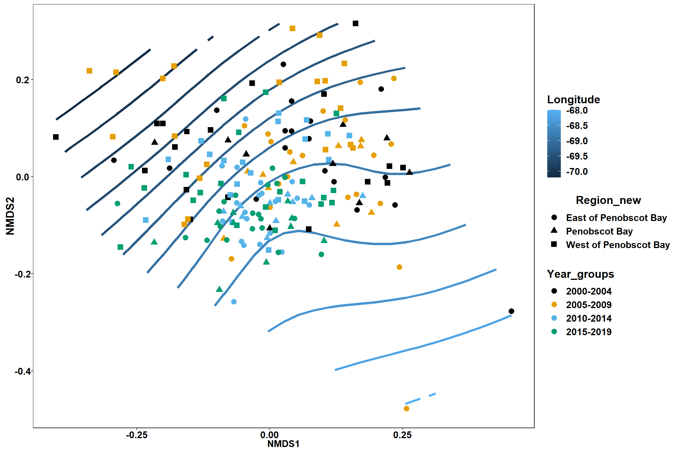
p1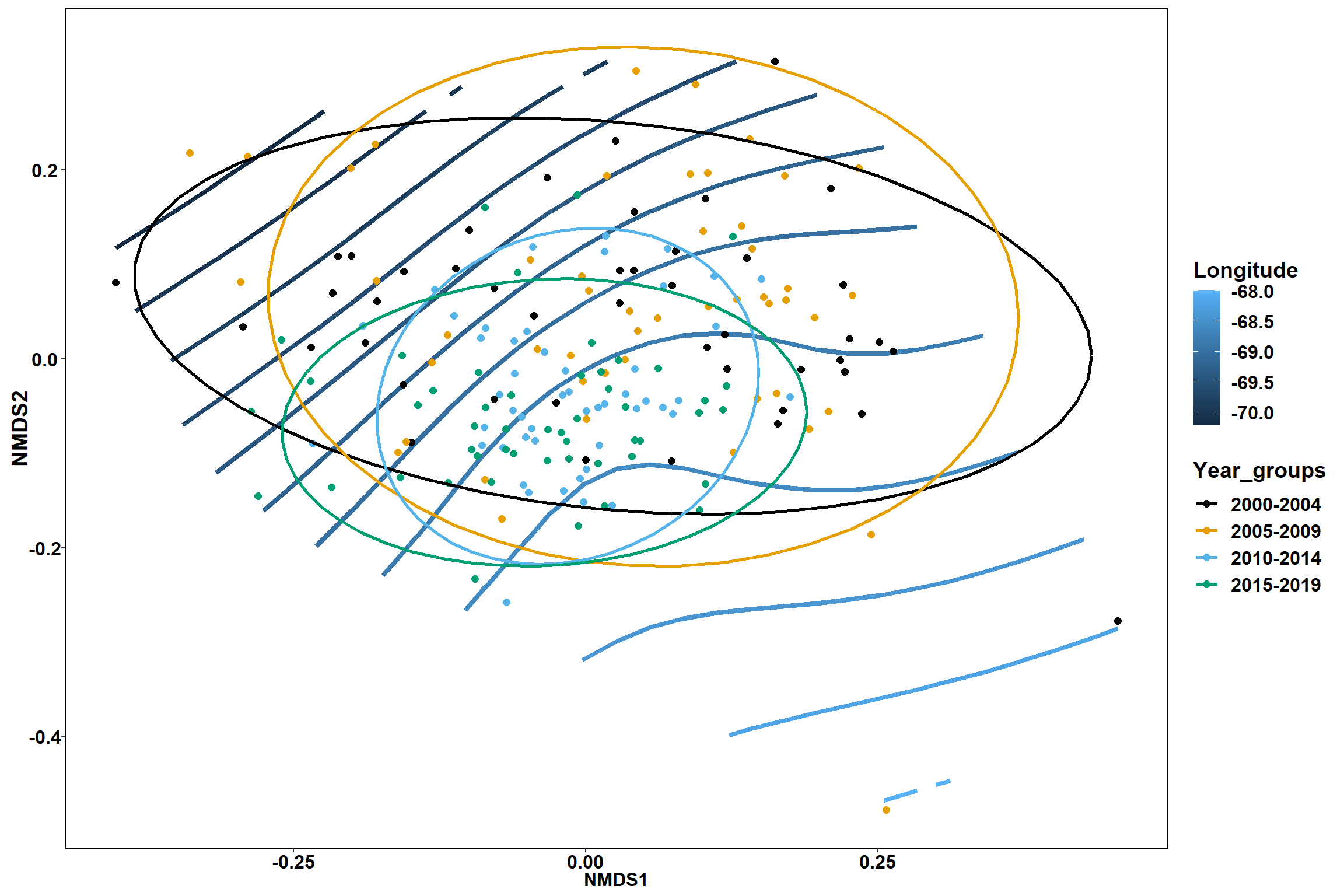
p2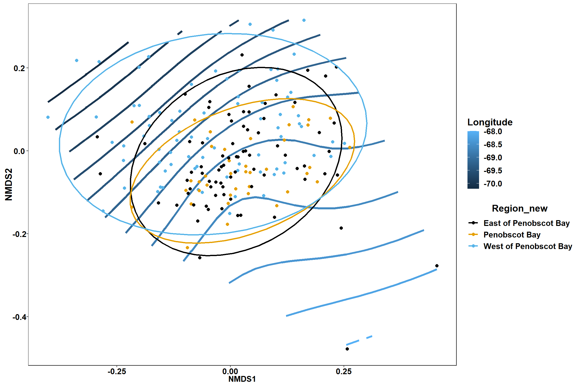
start depth
start_depth<-ordisurf(nmds, env$start_depth)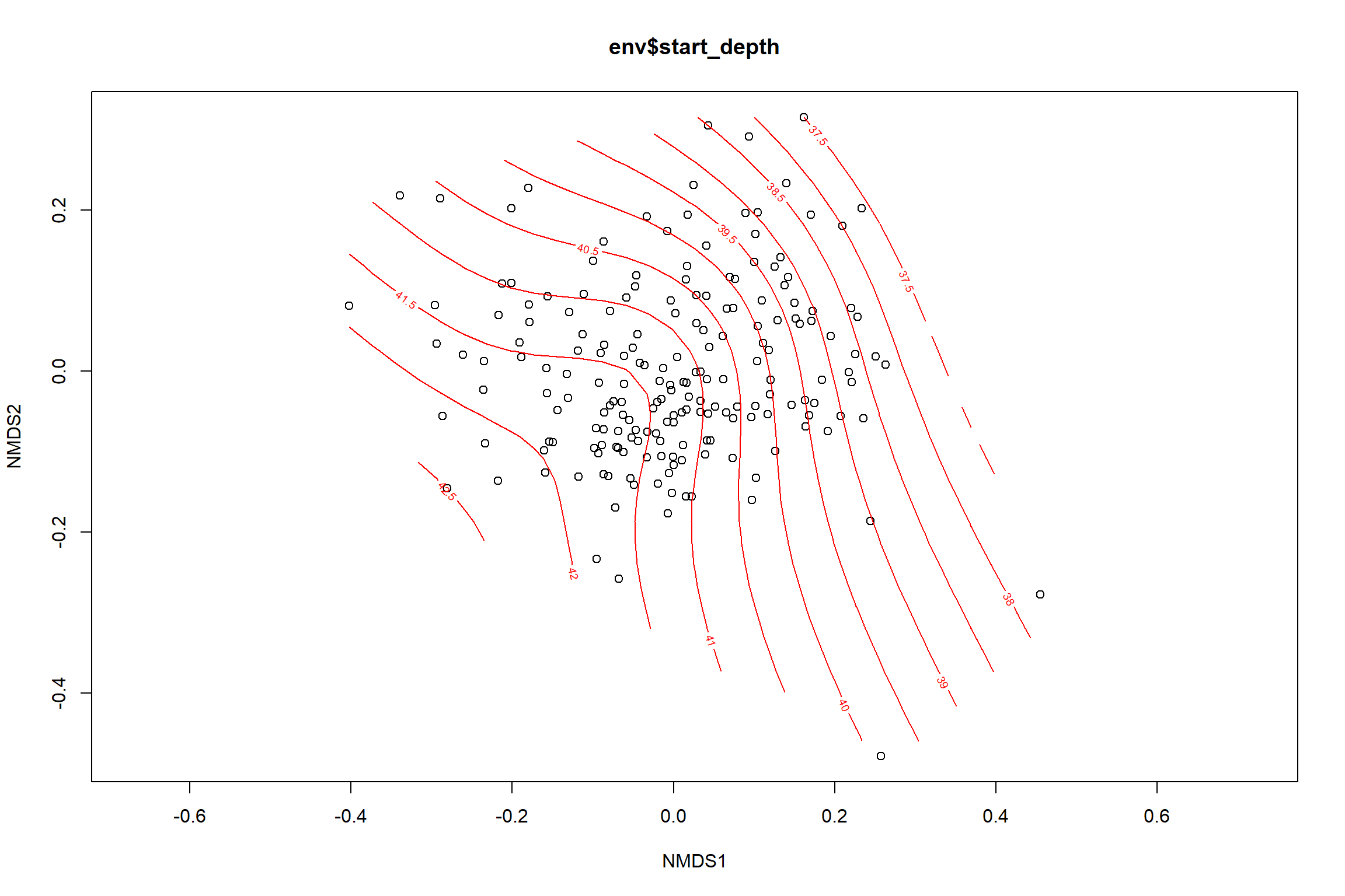
summary(start_depth)##
## Family: gaussian
## Link function: identity
##
## Formula:
## y ~ s(x1, x2, k = 10, bs = "tp", fx = FALSE)
##
## Parametric coefficients:
## Estimate Std. Error t value Pr(>|t|)
## (Intercept) 40.6472 0.3099 131.2 <2e-16 ***
## ---
## Signif. codes: 0 '***' 0.001 '**' 0.01 '*' 0.05 '.' 0.1 ' ' 1
##
## Approximate significance of smooth terms:
## edf Ref.df F p-value
## s(x1,x2) 3.619 9 1.791 0.000654 ***
## ---
## Signif. codes: 0 '***' 0.001 '**' 0.01 '*' 0.05 '.' 0.1 ' ' 1
##
## R-sq.(adj) = 0.0767 Deviance explained = 9.39%
## -REML = 565.42 Scale est. = 18.723 n = 195ordi.grid <- start_depth$grid #extracts the ordisurf object
#str(ordi.grid) #it's a list though - cannot be plotted as is
ordi.mite <- expand.grid(x = ordi.grid$x, y = ordi.grid$y) #get x and ys
ordi.mite$z <- as.vector(ordi.grid$z) #unravel the matrix for the z scores
contour.vals <- data.frame(na.omit(ordi.mite)) #gets rid of the nas
p <- ggplot()+
stat_contour(data = contour.vals, aes(x, y, z=z, color = ..level..),position="identity",size=1.5)+
labs(x = "NMDS1", y = "NMDS2", color="Depth")+
new_scale_color()+
geom_point(data = data.scores, aes(NMDS1, NMDS2, color=Year_groups, shape=Region_new), size = 3 )+ scale_color_colorblind()
p1 <- ggplot()+
stat_contour(data = contour.vals, aes(x, y, z=z, color = ..level..),position="identity",size=1.5)+
labs(x = "NMDS1", y = "NMDS2", color="Depth")+
new_scale_color()+
geom_point(data = data.scores, aes(NMDS1, NMDS2, color=Year_groups), size = 2 )+stat_ellipse(data=data.scores, aes(x=NMDS1, y=NMDS2, color=Year_groups),level = 0.95,size=1)+
scale_color_colorblind()
p2 <- ggplot()+
stat_contour(data = contour.vals, aes(x, y, z=z, color = ..level..),position="identity",size=1.5)+
labs(x = "NMDS1", y = "NMDS2", color="Depth")+
new_scale_color()+
geom_point(data = data.scores, aes(NMDS1, NMDS2, color=Region_new), size = 2 )+stat_ellipse(data=data.scores, aes(x=NMDS1, y=NMDS2, color=Region_new),level = 0.95,size=1)+
scale_color_colorblind()
p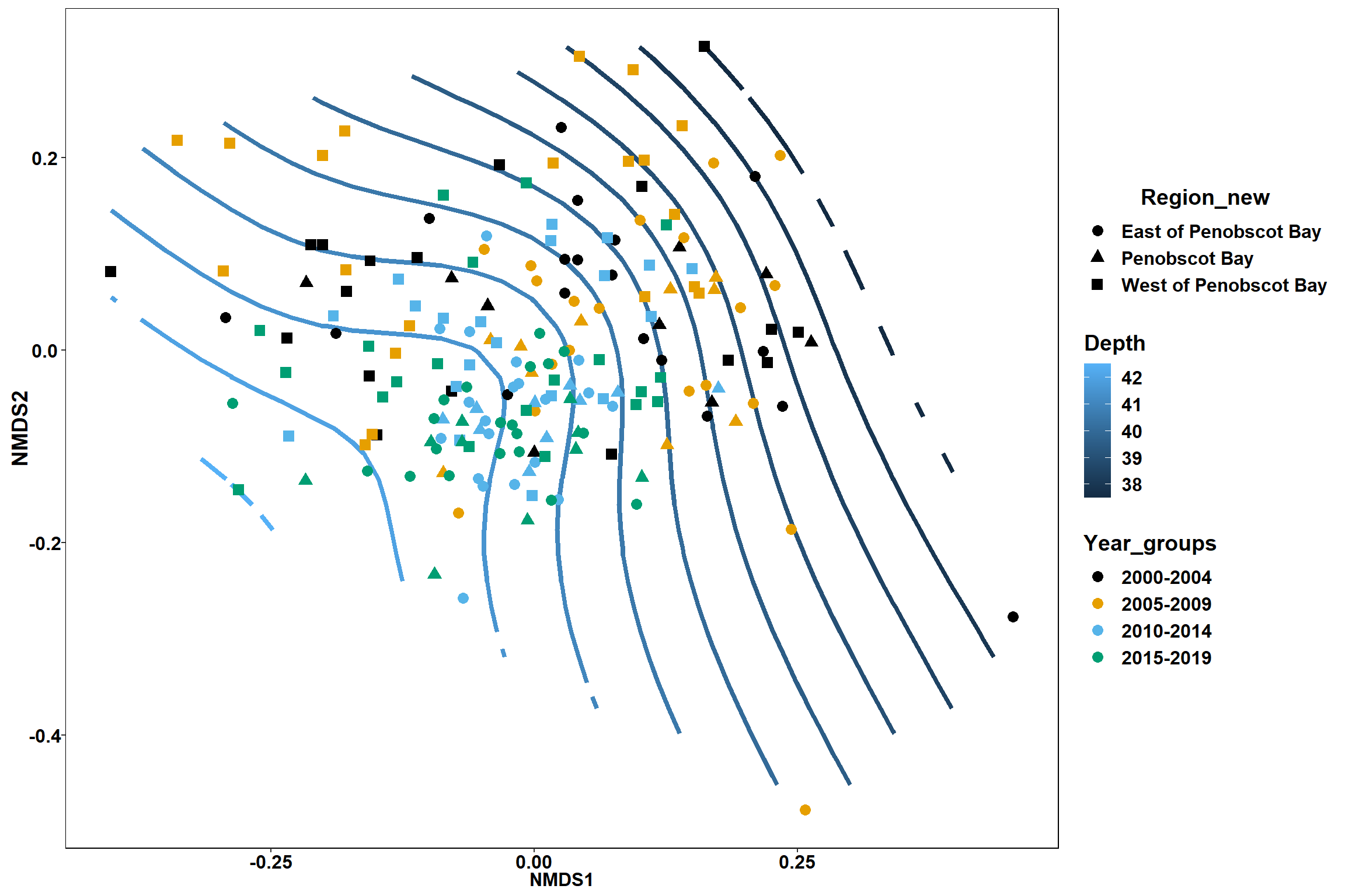
p1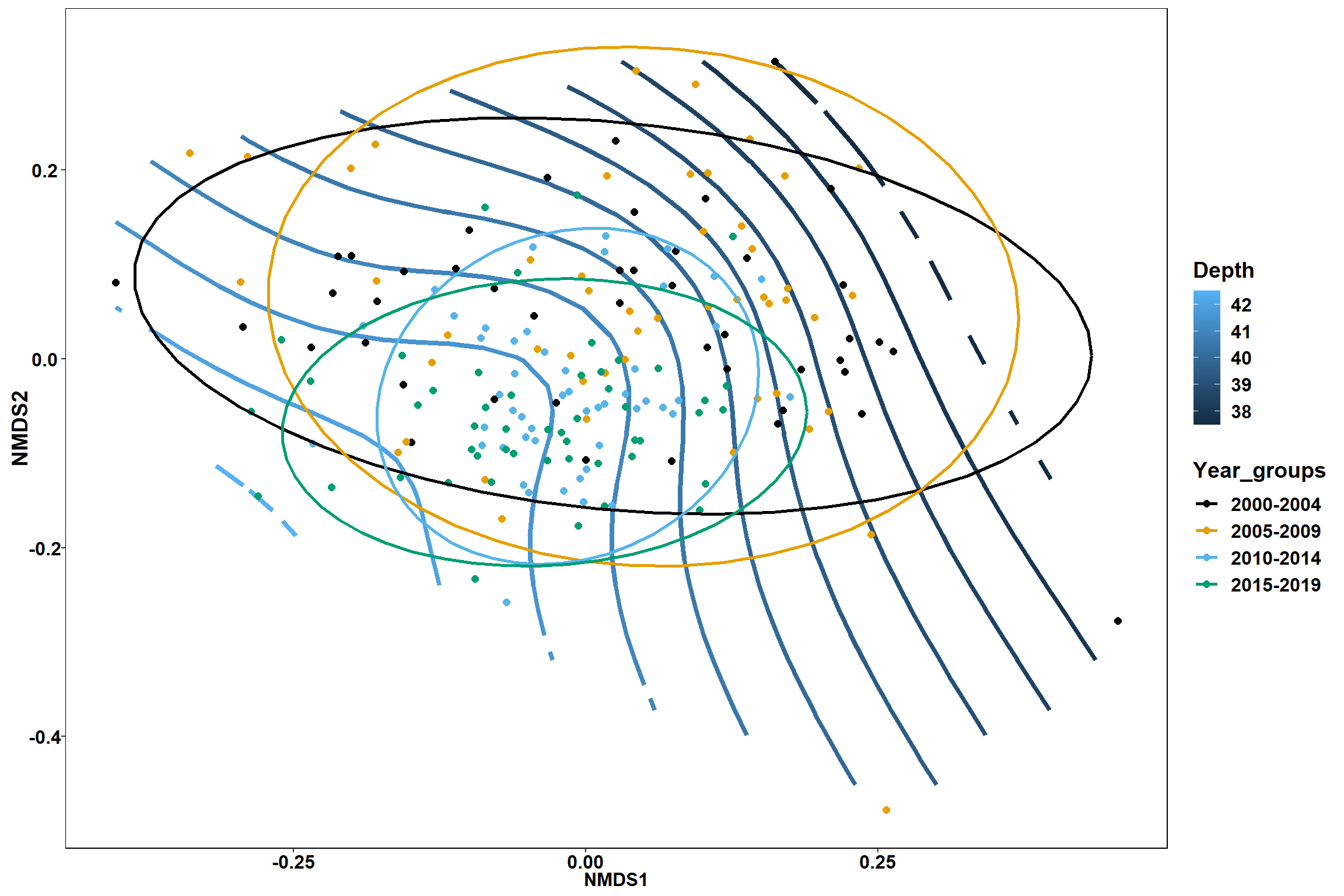
p2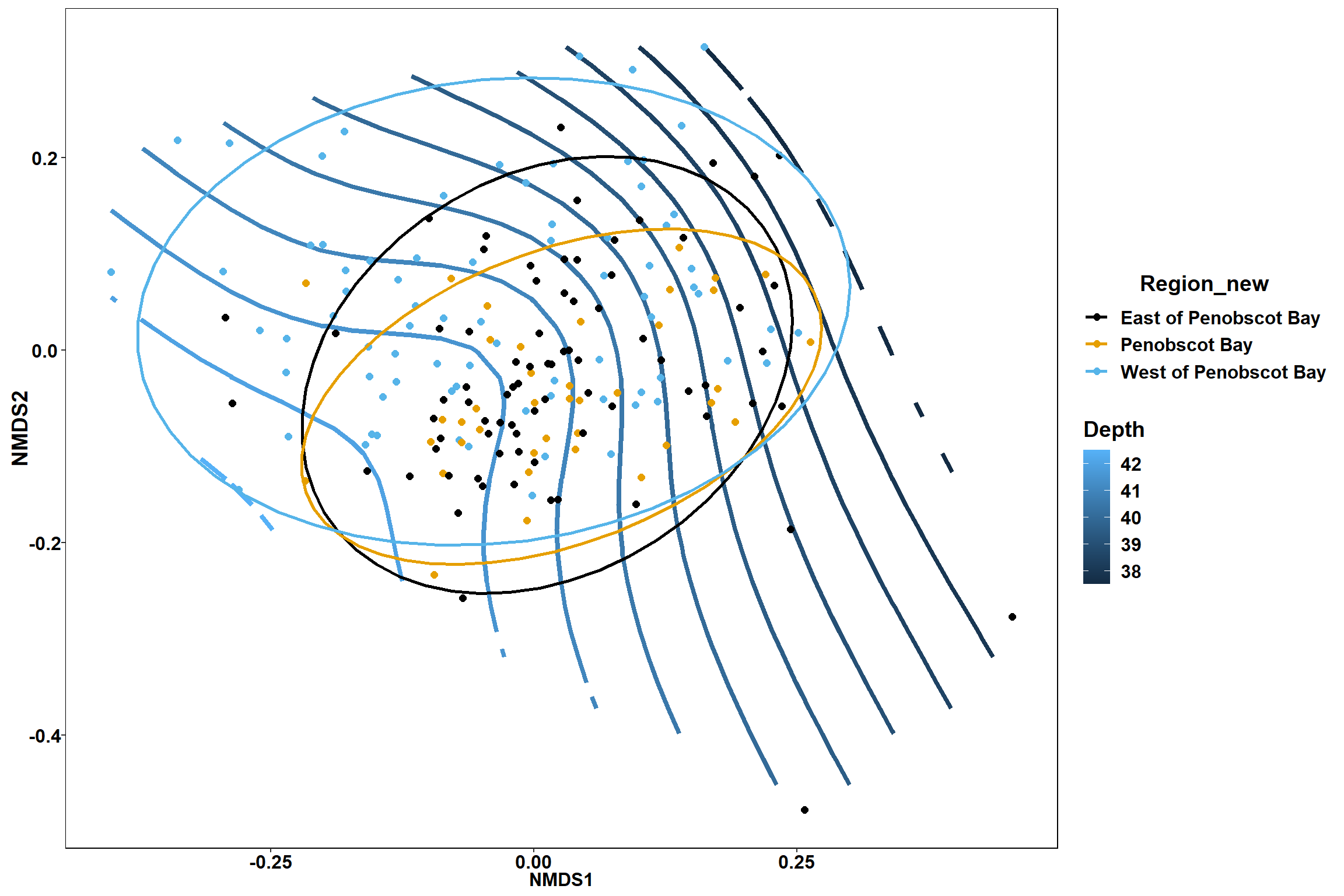
Funcitonal Group Abundance
NMDS
#load in data
trawl_data_arrange<-read.csv(here("Data/group_abundance_matrix.csv"))[-1]

trawl_data<-read.csv(here("Data/MaineDMR_Trawl_Survey_Tow_Data_2021-05-14.csv"))

all_Data<-group_by(trawl_data, Season, Year, Region)%>%
  filter(Year<2020)%>%
  summarise(start_lat=mean(Start_Latitude),start_long=mean(Start_Longitude),end_lat=mean(End_Latitude), end_long=mean(End_Longitude),start_depth=mean(Start_Depth_fathoms, na.rm=TRUE), end_depth=mean(End_Depth_fathoms, na.rm=TRUE), bottom_temp=mean(Bottom_WaterTemp_DegC, na.rm=TRUE), bottom_sal=mean(Bottom_Salinity, na.rm=TRUE),surface_temp=mean(Surface_WaterTemp_DegC, na.rm=TRUE), surface_sal=mean(Surface_Salinity, na.rm=TRUE))%>%
  full_join(trawl_data_arrange)%>%
  ungroup()

com<-select(all_Data,benthivore, benthos,piscivore,planktivore, undefined )

com<-vegdist(com, method="bray", na.rm=TRUE)

#convert com to a matrix
m_com = as.matrix(com)

set.seed(123)
nmds = metaMDS(m_com,k=2, distance = "bray", trymax = 200)
## Run 0 stress 0.1375071
## Run 1 stress 0.137507
## ... New best solution
## ... Procrustes: rmse 8.33793e-05 max resid 0.001121449
## ... Similar to previous best
## Run 2 stress 0.1404274
## Run 3 stress 0.1375071
## ... Procrustes: rmse 6.349328e-05 max resid 0.0006545503
## ... Similar to previous best
## Run 4 stress 0.1517021
## Run 5 stress 0.1404274
## Run 6 stress 0.1517024
## Run 7 stress 0.154412
## Run 8 stress 0.1375071
## ... Procrustes: rmse 3.188211e-05 max resid 0.0003404784
## ... Similar to previous best
## Run 9 stress 0.1404276
## Run 10 stress 0.1404275
## Run 11 stress 0.1375071
## ... Procrustes: rmse 8.125209e-05 max resid 0.001100816
## ... Similar to previous best
## Run 12 stress 0.1404274
## Run 13 stress 0.1517025
## Run 14 stress 0.1375068
## ... New best solution
## ... Procrustes: rmse 0.0003130745 max resid 0.00374505
## ... Similar to previous best
## Run 15 stress 0.1404274
## Run 16 stress 0.1375118
## ... Procrustes: rmse 0.0004065847 max resid 0.005198767
## ... Similar to previous best
## Run 17 stress 0.1404276
## Run 18 stress 0.137507
## ... Procrustes: rmse 0.0003082631 max resid 0.003739519
## ... Similar to previous best
## Run 19 stress 0.1544117
## Run 20 stress 0.1404274
## *** Solution reachednmds##
## Call:
## metaMDS(comm = m_com, distance = "bray", k = 2, trymax = 200)
##
## global Multidimensional Scaling using monoMDS
##
## Data: m_com
## Distance: user supplied
##
## Dimensions: 2
## Stress: 0.1375068
## Stress type 1, weak ties
## Two convergent solutions found after 20 tries
## Scaling: centring, PC rotation
## Species: scores missingEnvfit
env<-select(all_Data, start_lat, start_long, end_lat, end_long,start_depth, end_depth, bottom_temp, bottom_sal, surface_temp, surface_sal)

en<-envfit(nmds, env, permutations=999, na.rm=TRUE)
en
##
## ***VECTORS
##
## NMDS1 NMDS2 r2 Pr(>r)
## start_lat 0.43552 -0.90018 0.0033 0.750
## start_long -0.98594 -0.16711 0.0017 0.861
## end_lat 0.42320 -0.90604 0.0034 0.748
## end_long -0.98374 -0.17959 0.0017 0.859
## start_depth -0.99993 -0.01194 0.0393 0.035 *
## end_depth -0.99999 0.00455 0.0341 0.045 *
## bottom_temp -0.63753 -0.77042 0.0917 0.001 ***
## bottom_sal -0.87298 -0.48776 0.0905 0.001 ***
## surface_temp -0.82126 -0.57056 0.1043 0.001 ***
## surface_sal -0.56102 -0.82780 0.0004 0.970
## ---
## Signif. codes: 0 '***' 0.001 '**' 0.01 '*' 0.05 '.' 0.1 ' ' 1
## Permutation: free
## Number of permutations: 999
##
## 5 observations deleted due to missingnessplot(nmds)
plot(en)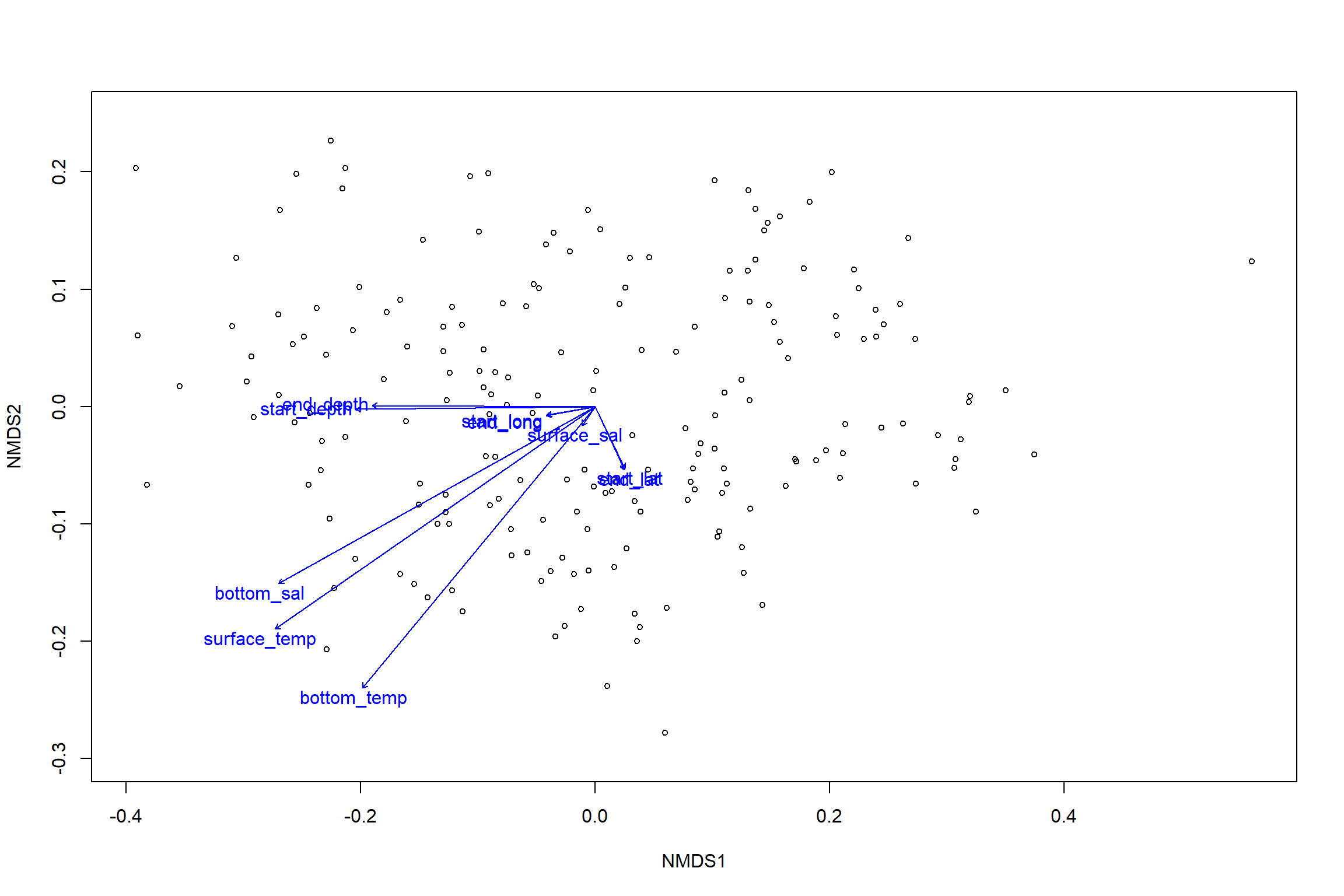
en_coord_cont = as.data.frame(scores(en, "vectors")) * ordiArrowMul(en)
en_coord_cat = as.data.frame(scores(en, "factors")) * ordiArrowMul(en)

#extract NMDS scores for ggplot
data.scores = as.data.frame(scores(nmds))
#add columns to data frame
data.scores$Region = all_Data$Region
data.scores$Year = all_Data$Year
data.scores$Season= all_Data$Season
data.scores$Year_groups= all_Data$YEAR_GROUPS
data.scores$Year_decades= all_Data$YEAR_DECADES
data.scores$Region_new=all_Data$REGION_NEW
data.scores$Region_year=all_Data$REGION_YEAR
data.scores$Season_year=all_Data$SEASON_YEAR

p<- ggplot()+
     geom_point(data = data.scores, aes(x = NMDS1, y = NMDS2, color=Year_groups, shape=Region_new), size = 4) +
  scale_color_colorblind()+
        geom_segment(data=en_coord_cont, aes(x = 0, y = 0, xend = NMDS1, yend = NMDS2), size =1.5, alpha = 0.5)+
   geom_text(data = en_coord_cont, aes(x = NMDS1, y = NMDS2), size=5,
       fontface = "bold", label = row.names(en_coord_cont))+
    theme(axis.title = element_text(size = 16, face = "bold"),
       panel.background = element_blank(), panel.border = element_rect(fill = NA),
       axis.ticks = element_blank(), axis.text = element_blank(), legend.key = element_blank(),
       legend.title = element_text(size = 16, face = "bold"),
       legend.text = element_text(size = 16))


p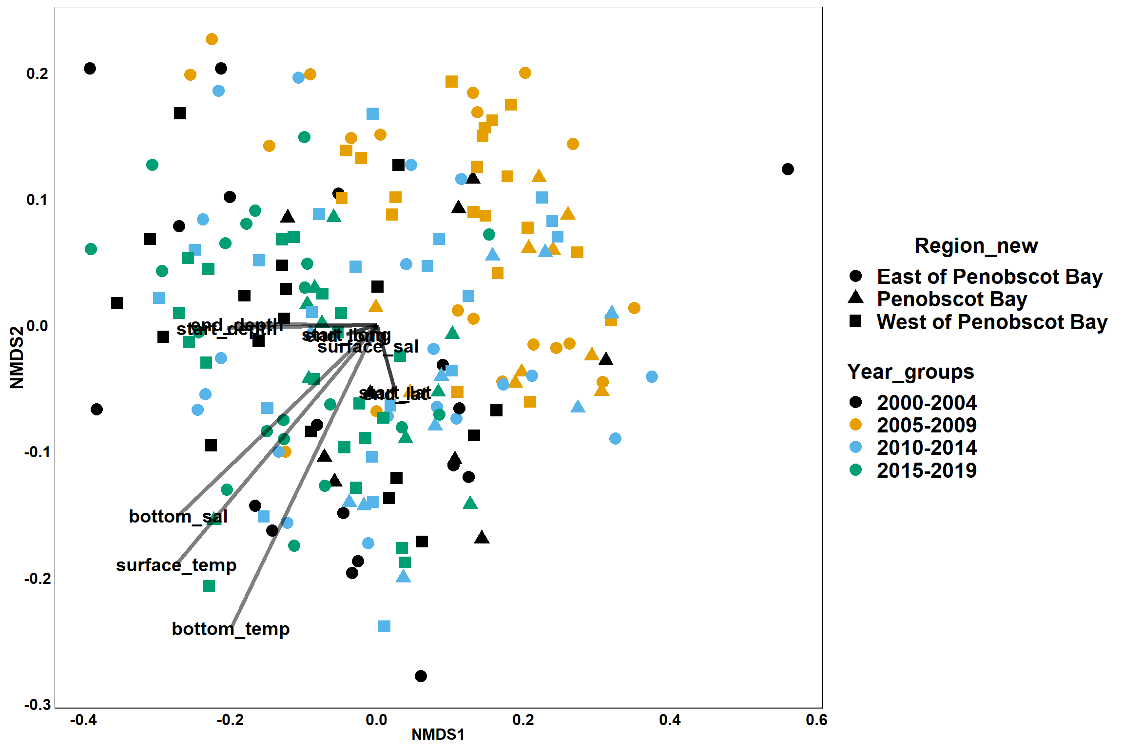
Region groups
p_region<- ggplot()+
     geom_point(data = data.scores, aes(x = NMDS1, y = NMDS2, color=Region_new), size = 4) +
  scale_color_colorblind()+
        geom_segment(data=en_coord_cont, aes(x = 0, y = 0, xend = NMDS1, yend = NMDS2), size =1.5, alpha = 0.5)+
   geom_text(data = en_coord_cont, aes(x = NMDS1, y = NMDS2), size=5,
       fontface = "bold", label = row.names(en_coord_cont))+
  stat_ellipse(data=data.scores, aes(x=NMDS1, y=NMDS2, color=Region_new),level = 0.95,size=1)+
  theme(axis.title = element_text(size = 16, face = "bold"),
       panel.background = element_blank(), panel.border = element_rect(fill = NA),
       axis.ticks = element_blank(), axis.text = element_blank(), legend.key = element_blank(),
       legend.title = element_text(size = 16, face = "bold"),
       legend.text = element_text(size = 16))


p_region
Year groups
p_year<- ggplot()+
     geom_point(data = data.scores, aes(x = NMDS1, y = NMDS2, color=Year_groups), size = 4) +
  scale_color_colorblind()+
        geom_segment(data=en_coord_cont, aes(x = 0, y = 0, xend = NMDS1, yend = NMDS2), size =1.5, alpha = 0.5)+
   geom_text(data = en_coord_cont, aes(x = NMDS1, y = NMDS2), size=5,
       fontface = "bold", label = row.names(en_coord_cont))+
  stat_ellipse(data=data.scores, aes(x=NMDS1, y=NMDS2, color=Year_groups),level = 0.95,size=1)+
  theme(axis.title = element_text(size = 16, face = "bold"),
       panel.background = element_blank(), panel.border = element_rect(fill = NA),
       axis.ticks = element_blank(), axis.text = element_blank(), legend.key = element_blank(),
       legend.title = element_text(size = 16, face = "bold"),
       legend.text = element_text(size = 16))

p_year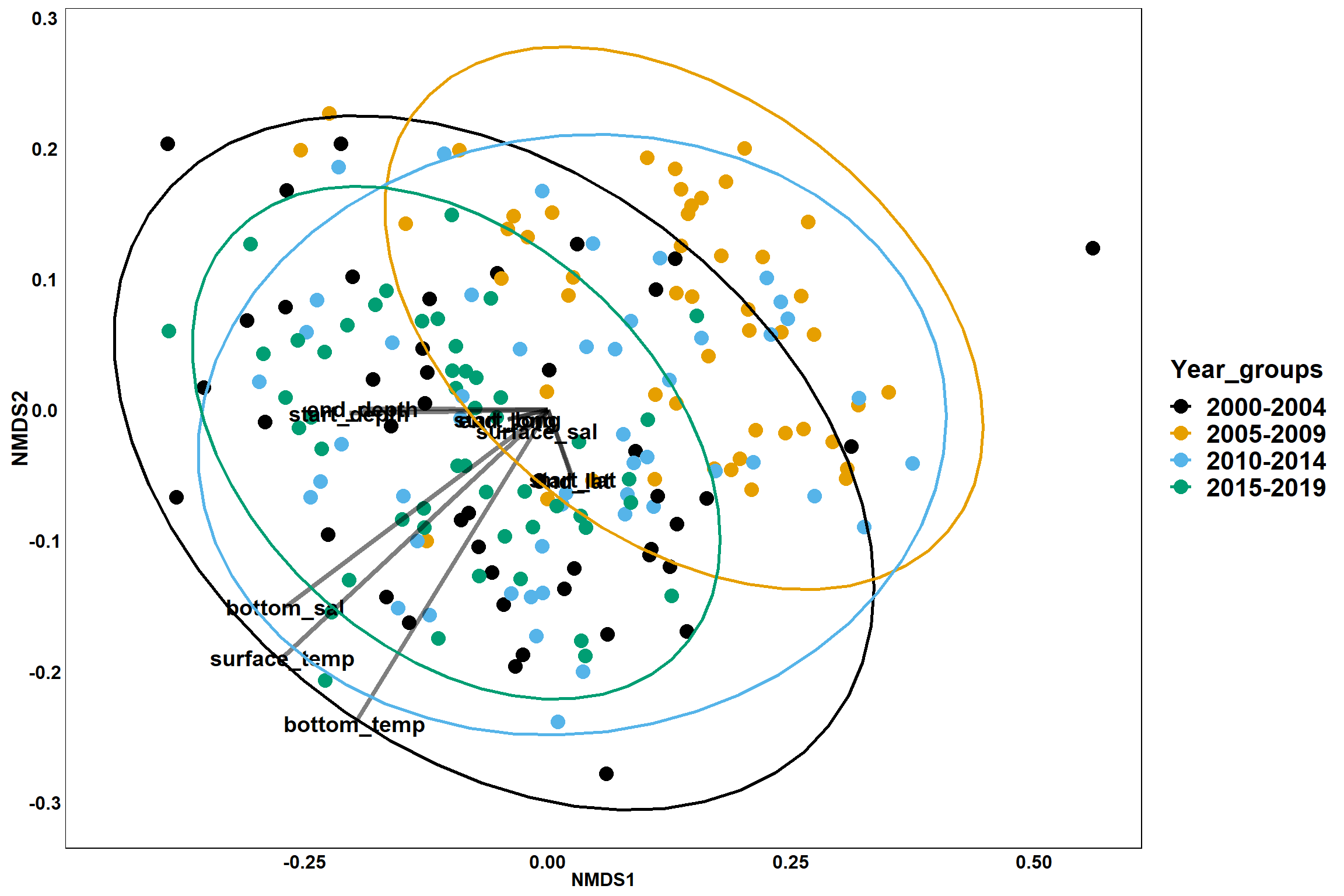
GAM contours for environmental effects
Bottom temperature
bottom_temp<-ordisurf(nmds, env$bottom_temp)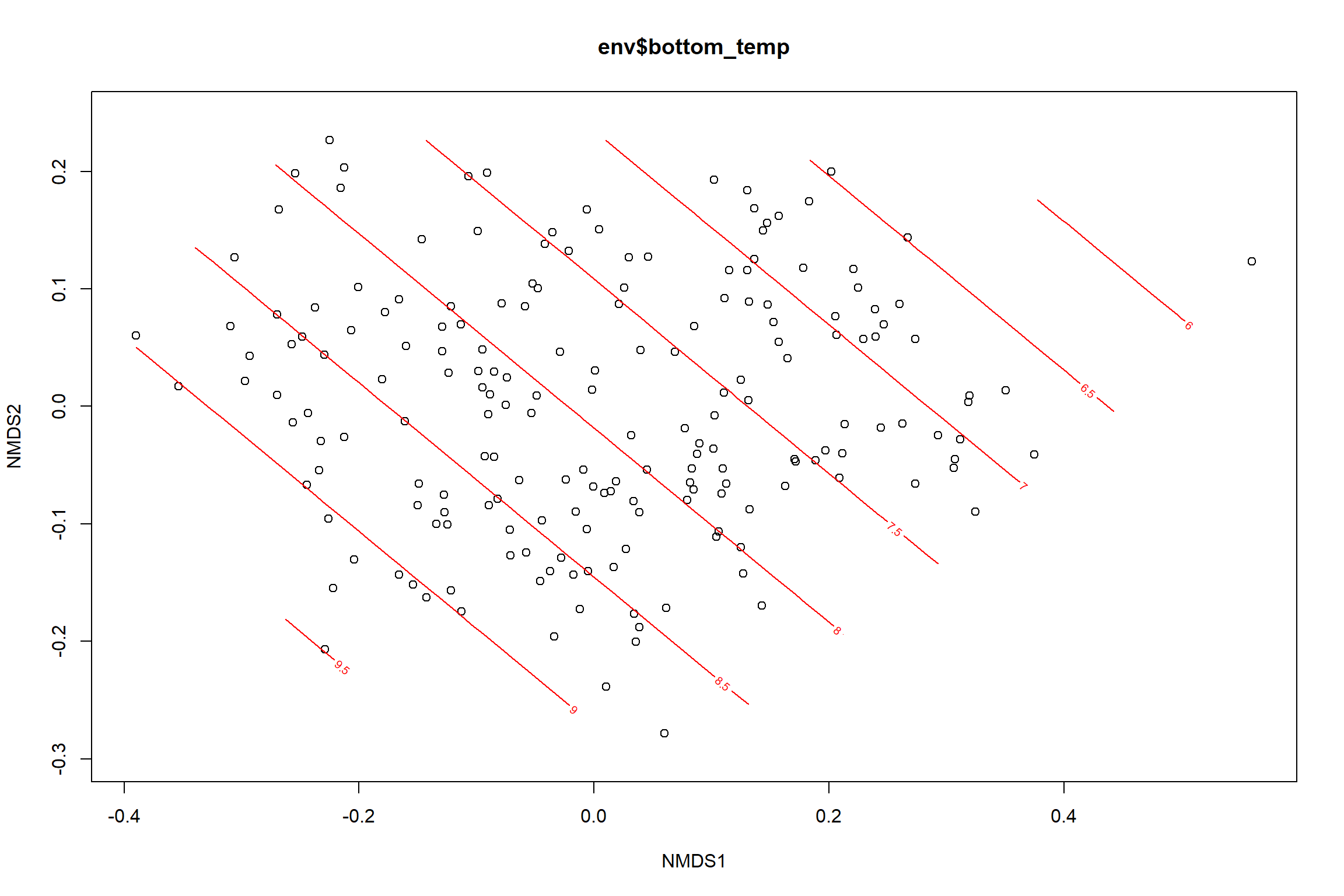
summary(bottom_temp)##
## Family: gaussian
## Link function: identity
##
## Formula:
## y ~ s(x1, x2, k = 10, bs = "tp", fx = FALSE)
##
## Parametric coefficients:
## Estimate Std. Error t value Pr(>|t|)
## (Intercept) 7.9053 0.1806 43.76 <2e-16 ***
## ---
## Signif. codes: 0 '***' 0.001 '**' 0.01 '*' 0.05 '.' 0.1 ' ' 1
##
## Approximate significance of smooth terms:
## edf Ref.df F p-value
## s(x1,x2) 1.786 9 1.876 0.000123 ***
## ---
## Signif. codes: 0 '***' 0.001 '**' 0.01 '*' 0.05 '.' 0.1 ' ' 1
##
## R-sq.(adj) = 0.082 Deviance explained = 9.07%
## -REML = 445.45 Scale est. = 6.1995 n = 190ordi.grid <- bottom_temp$grid #extracts the ordisurf object
#str(ordi.grid) #it's a list though - cannot be plotted as is
ordi.mite <- expand.grid(x = ordi.grid$x, y = ordi.grid$y) #get x and ys
ordi.mite$z <- as.vector(ordi.grid$z) #unravel the matrix for the z scores
contour.vals <- data.frame(na.omit(ordi.mite)) #gets rid of the nas
p <- ggplot()+
stat_contour(data = contour.vals, aes(x, y, z=z, color = ..level..),position="identity",size=1.5)+
labs(x = "NMDS1", y = "NMDS2", color="Bottom Temperature")+
new_scale_color()+
geom_point(data = data.scores, aes(NMDS1, NMDS2, color=Year_groups, shape=Region_new), size = 3 )+ scale_color_colorblind()
p1 <- ggplot()+
stat_contour(data = contour.vals, aes(x, y, z=z, color = ..level..),position="identity",size=1.5)+
labs(x = "NMDS1", y = "NMDS2", color="Bottom Temperature")+
new_scale_color()+
geom_point(data = data.scores, aes(NMDS1, NMDS2, color=Year_groups), size = 2 )+ stat_ellipse(data=data.scores, aes(x=NMDS1, y=NMDS2, color=Year_groups),level = 0.95,size=1)+
scale_color_colorblind()
p2 <- ggplot()+
stat_contour(data = contour.vals, aes(x, y, z=z, color = ..level..),position="identity",size=1.5)+
labs(x = "NMDS1", y = "NMDS2", color="Bottom Temperature")+
new_scale_color()+
geom_point(data = data.scores, aes(NMDS1, NMDS2, color=Region_new), size = 2 )+
stat_ellipse(data=data.scores, aes(x=NMDS1, y=NMDS2, color=Region_new),level = 0.95,size=1)+
scale_color_colorblind()
p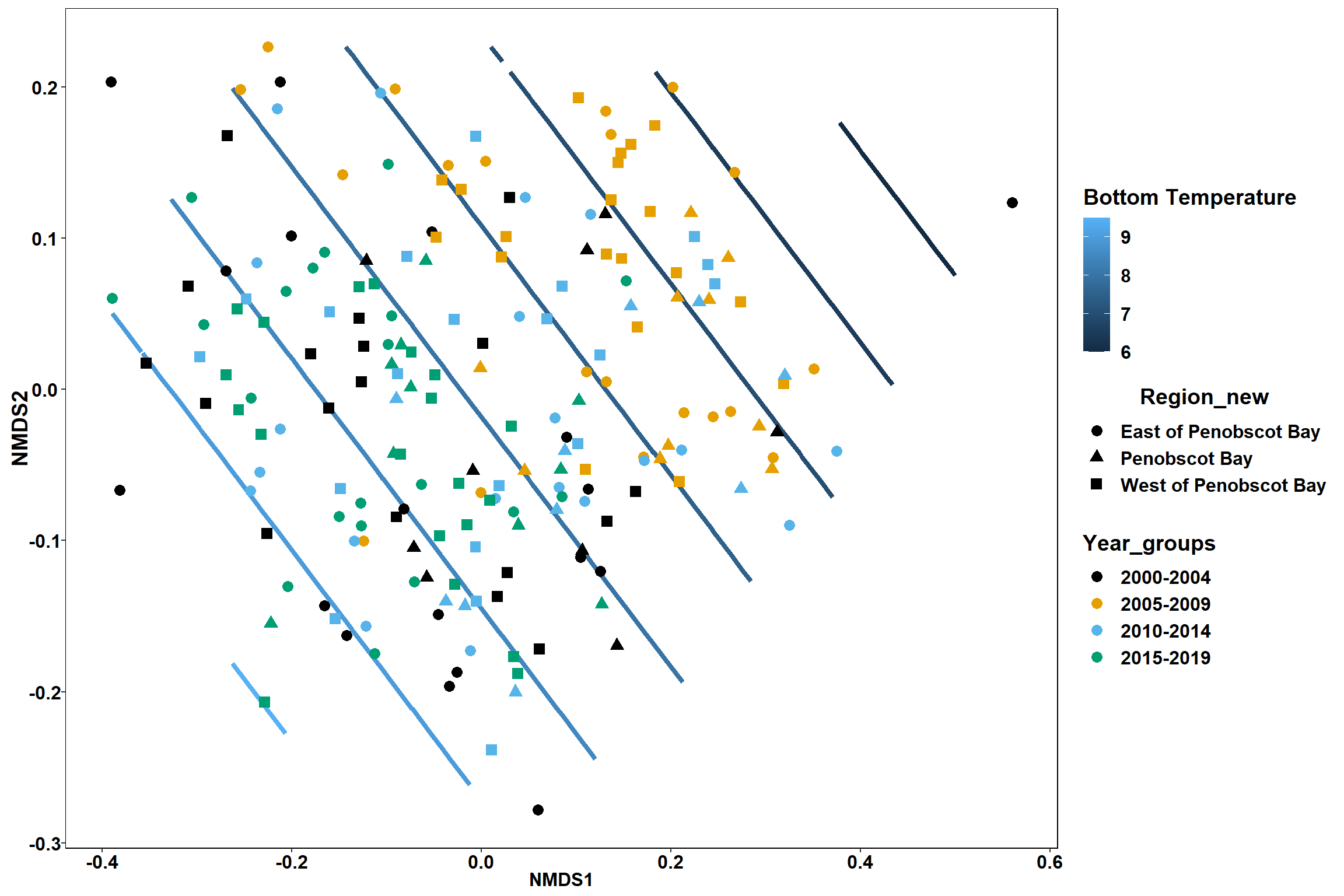
p1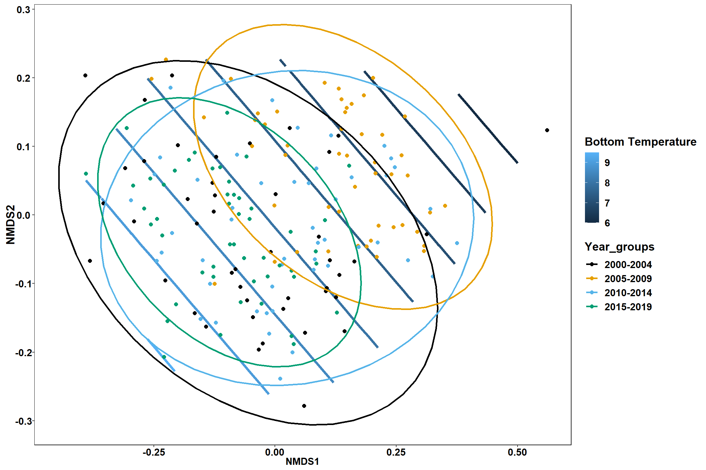
p2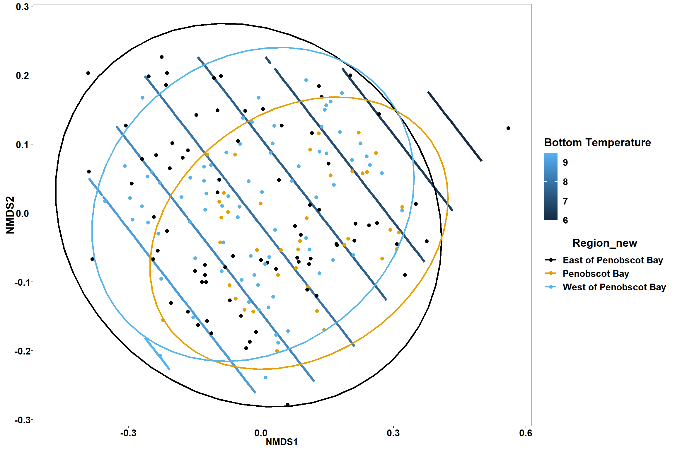
Surface temperature
surface_temp<-ordisurf(nmds, env$surface_temp)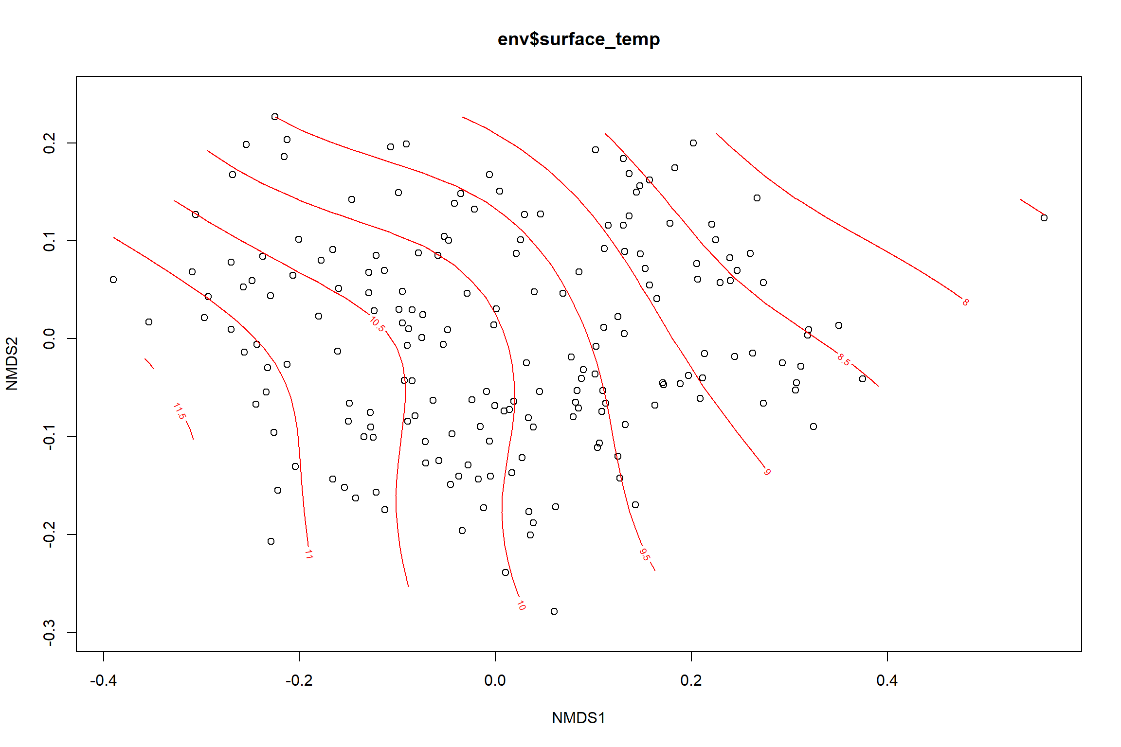
summary(surface_temp)##
## Family: gaussian
## Link function: identity
##
## Formula:
## y ~ s(x1, x2, k = 10, bs = "tp", fx = FALSE)
##
## Parametric coefficients:
## Estimate Std. Error t value Pr(>|t|)
## (Intercept) 9.7700 0.1866 52.37 <2e-16 ***
## ---
## Signif. codes: 0 '***' 0.001 '**' 0.01 '*' 0.05 '.' 0.1 ' ' 1
##
## Approximate significance of smooth terms:
## edf Ref.df F p-value
## s(x1,x2) 3.931 9 2.548 3.44e-05 ***
## ---
## Signif. codes: 0 '***' 0.001 '**' 0.01 '*' 0.05 '.' 0.1 ' ' 1
##
## R-sq.(adj) = 0.108 Deviance explained = 12.7%
## -REML = 453.05 Scale est. = 6.6138 n = 190ordi.grid <- surface_temp$grid #extracts the ordisurf object
#str(ordi.grid) #it's a list though - cannot be plotted as is
ordi.mite <- expand.grid(x = ordi.grid$x, y = ordi.grid$y) #get x and ys
ordi.mite$z <- as.vector(ordi.grid$z) #unravel the matrix for the z scores
contour.vals <- data.frame(na.omit(ordi.mite)) #gets rid of the nas
p <- ggplot()+
stat_contour(data = contour.vals, aes(x, y, z=z, color = ..level..),position="identity",size=1.5)+
labs(x = "NMDS1", y = "NMDS2", color="Surface Temperature")+
new_scale_color()+
geom_point(data = data.scores, aes(NMDS1, NMDS2, color=Year_groups, shape=Region_new), size = 3 )+ scale_color_colorblind()
p1 <- ggplot()+
stat_contour(data = contour.vals, aes(x, y, z=z, color = ..level..),position="identity",size=1.5)+
labs(x = "NMDS1", y = "NMDS2", color="Surface Temperature")+
new_scale_color()+
geom_point(data = data.scores, aes(NMDS1, NMDS2, color=Year_groups), size = 2 )+stat_ellipse(data=data.scores, aes(x=NMDS1, y=NMDS2, color=Year_groups),level = 0.95,size=1)+
scale_color_colorblind()
p2 <- ggplot()+
stat_contour(data = contour.vals, aes(x, y, z=z, color = ..level..),position="identity",size=1.5)+
labs(x = "NMDS1", y = "NMDS2", color="Surface Temperature")+
new_scale_color()+
geom_point(data = data.scores, aes(NMDS1, NMDS2, color=Region_new), size = 2 )+stat_ellipse(data=data.scores, aes(x=NMDS1, y=NMDS2, color=Region_new),level = 0.95,size=1)+
scale_color_colorblind()
p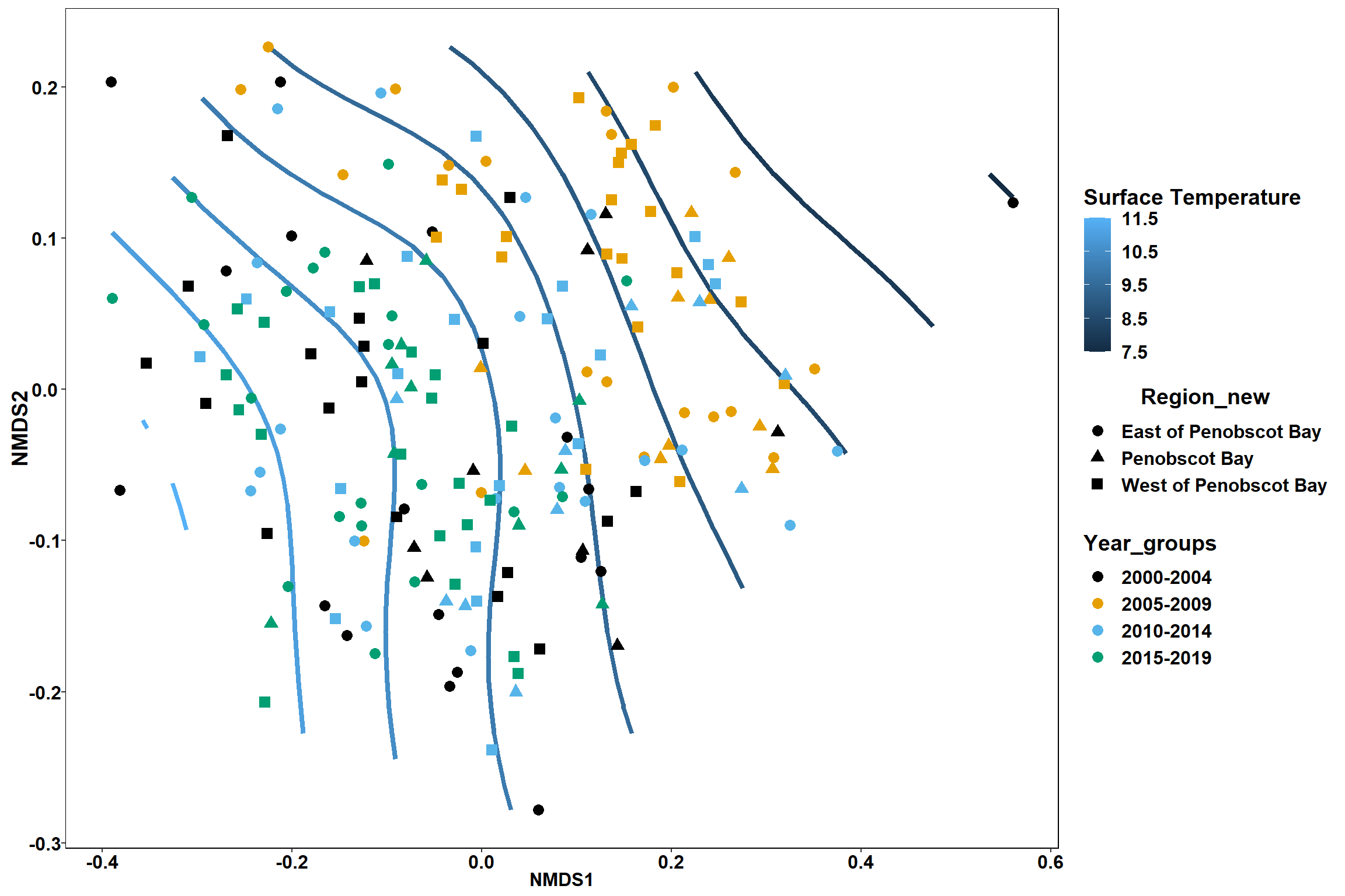
p1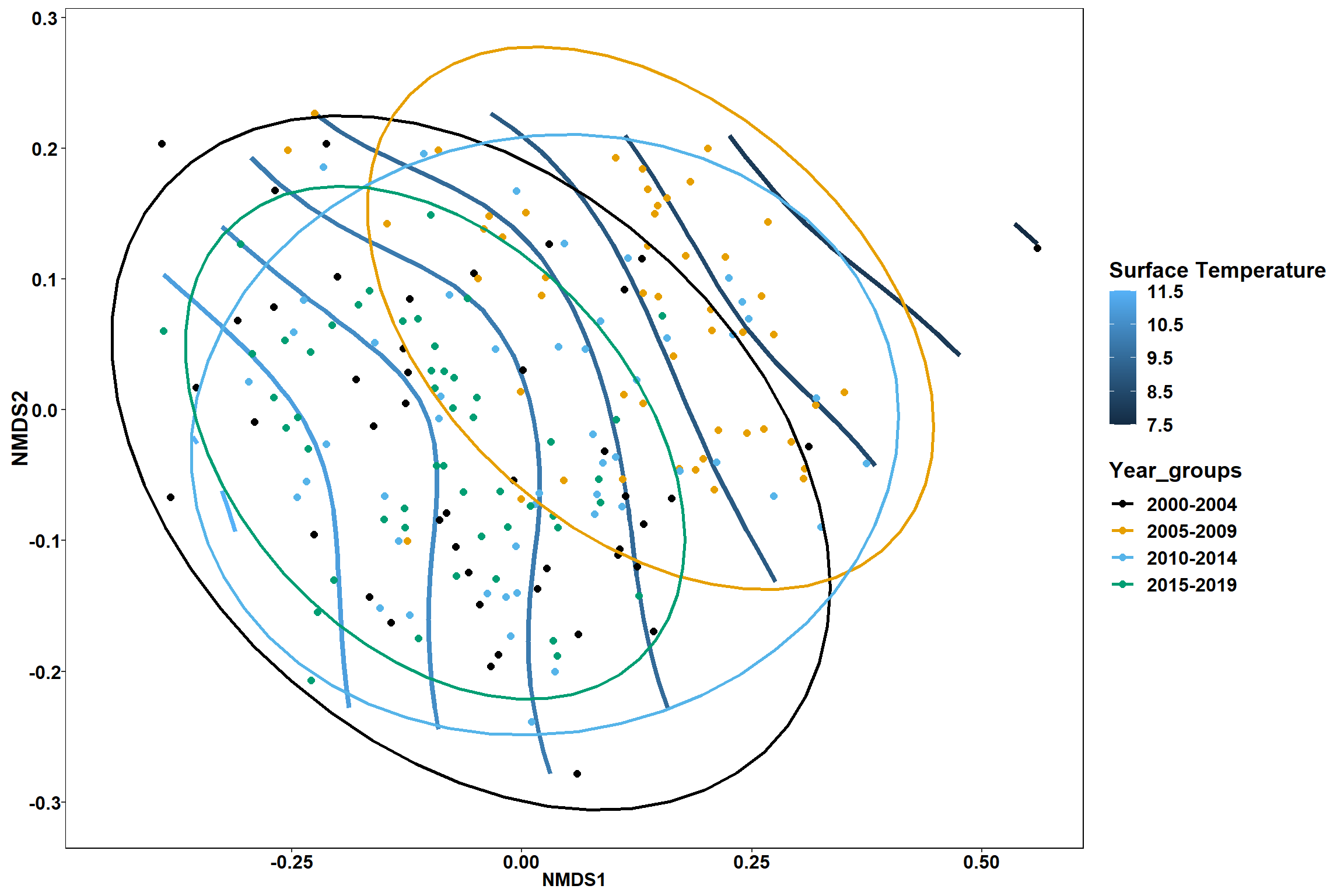
p2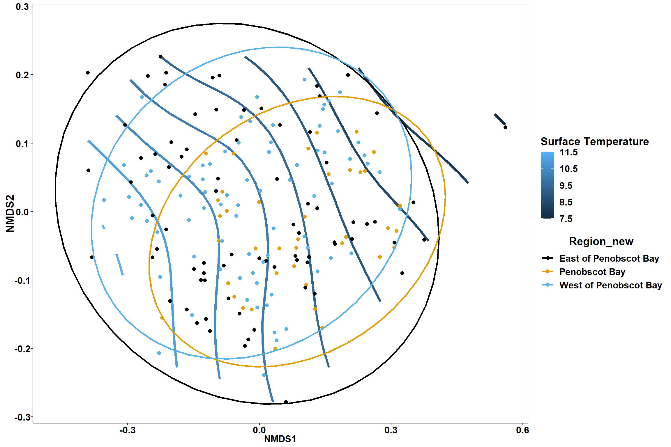
Bottom salinity
bottom_sal<-ordisurf(nmds, env$bottom_sal)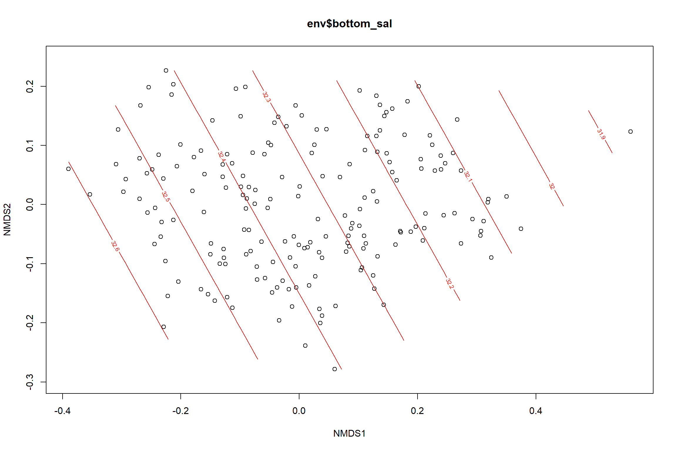
summary(bottom_sal)##
## Family: gaussian
## Link function: identity
##
## Formula:
## y ~ s(x1, x2, k = 10, bs = "tp", fx = FALSE)
##
## Parametric coefficients:
## Estimate Std. Error t value Pr(>|t|)
## (Intercept) 32.33134 0.03573 904.8 <2e-16 ***
## ---
## Signif. codes: 0 '***' 0.001 '**' 0.01 '*' 0.05 '.' 0.1 ' ' 1
##
## Approximate significance of smooth terms:
## edf Ref.df F p-value
## s(x1,x2) 1.784 9 1.845 0.00014 ***
## ---
## Signif. codes: 0 '***' 0.001 '**' 0.01 '*' 0.05 '.' 0.1 ' ' 1
##
## R-sq.(adj) = 0.0808 Deviance explained = 8.94%
## -REML = 139.19 Scale est. = 0.24262 n = 190ordi.grid <- bottom_sal$grid #extracts the ordisurf object
#str(ordi.grid) #it's a list though - cannot be plotted as is
ordi.mite <- expand.grid(x = ordi.grid$x, y = ordi.grid$y) #get x and ys
ordi.mite$z <- as.vector(ordi.grid$z) #unravel the matrix for the z scores
contour.vals <- data.frame(na.omit(ordi.mite)) #gets rid of the nas
p <- ggplot()+
stat_contour(data = contour.vals, aes(x, y, z=z, color = ..level..),position="identity",size=1.5)+
labs(x = "NMDS1", y = "NMDS2", color="Bottom Salinity")+
new_scale_color()+
geom_point(data = data.scores, aes(NMDS1, NMDS2, color=Year_groups, shape=Region_new), size = 3 )+ scale_color_colorblind()
p1 <- ggplot()+
stat_contour(data = contour.vals, aes(x, y, z=z, color = ..level..),position="identity",size=1.5)+
labs(x = "NMDS1", y = "NMDS2", color="Bottom Salinity")+
new_scale_color()+
geom_point(data = data.scores, aes(NMDS1, NMDS2, color=Year_groups), size = 2 )+ stat_ellipse(data=data.scores, aes(x=NMDS1, y=NMDS2, color=Year_groups),level = 0.95,size=1)+
scale_color_colorblind()
p2 <- ggplot()+
stat_contour(data = contour.vals, aes(x, y, z=z, color = ..level..),position="identity",size=1.5)+
labs(x = "NMDS1", y = "NMDS2", color="Bottom Salinity")+
new_scale_color()+
geom_point(data = data.scores, aes(NMDS1, NMDS2, color=Region_new), size = 2 )+stat_ellipse(data=data.scores, aes(x=NMDS1, y=NMDS2, color=Region_new),level = 0.95,size=1)+
scale_color_colorblind()
p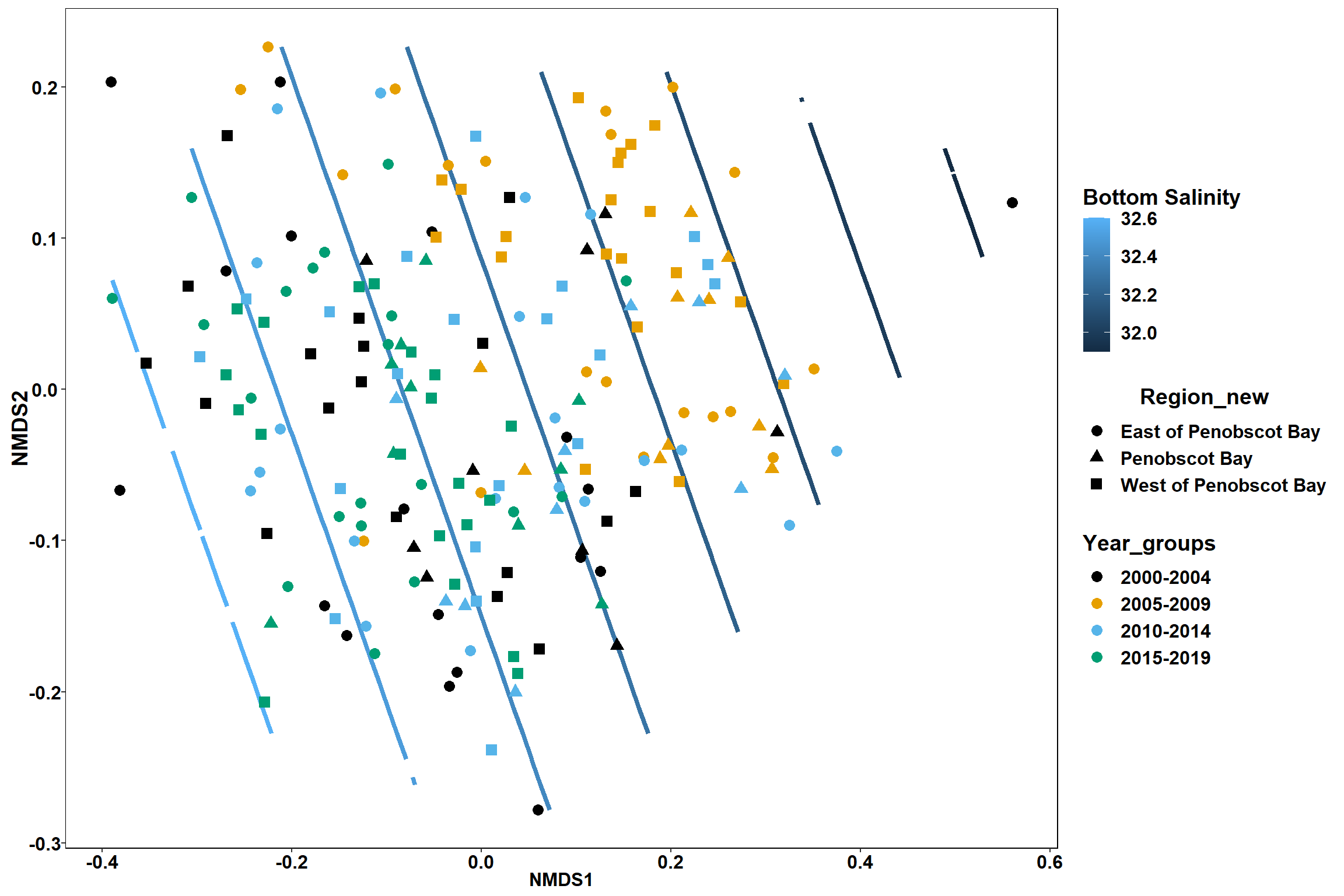
p1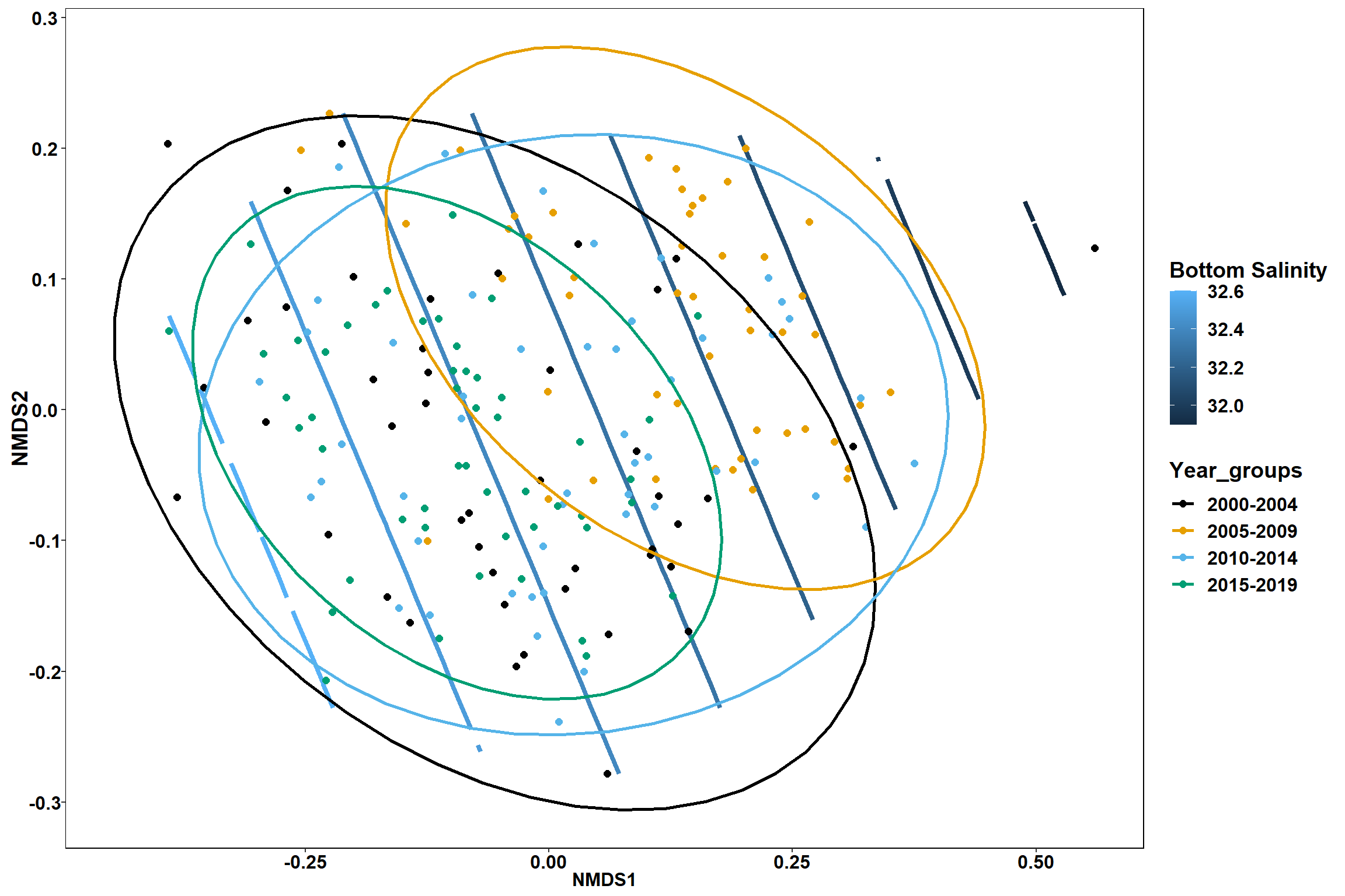
p2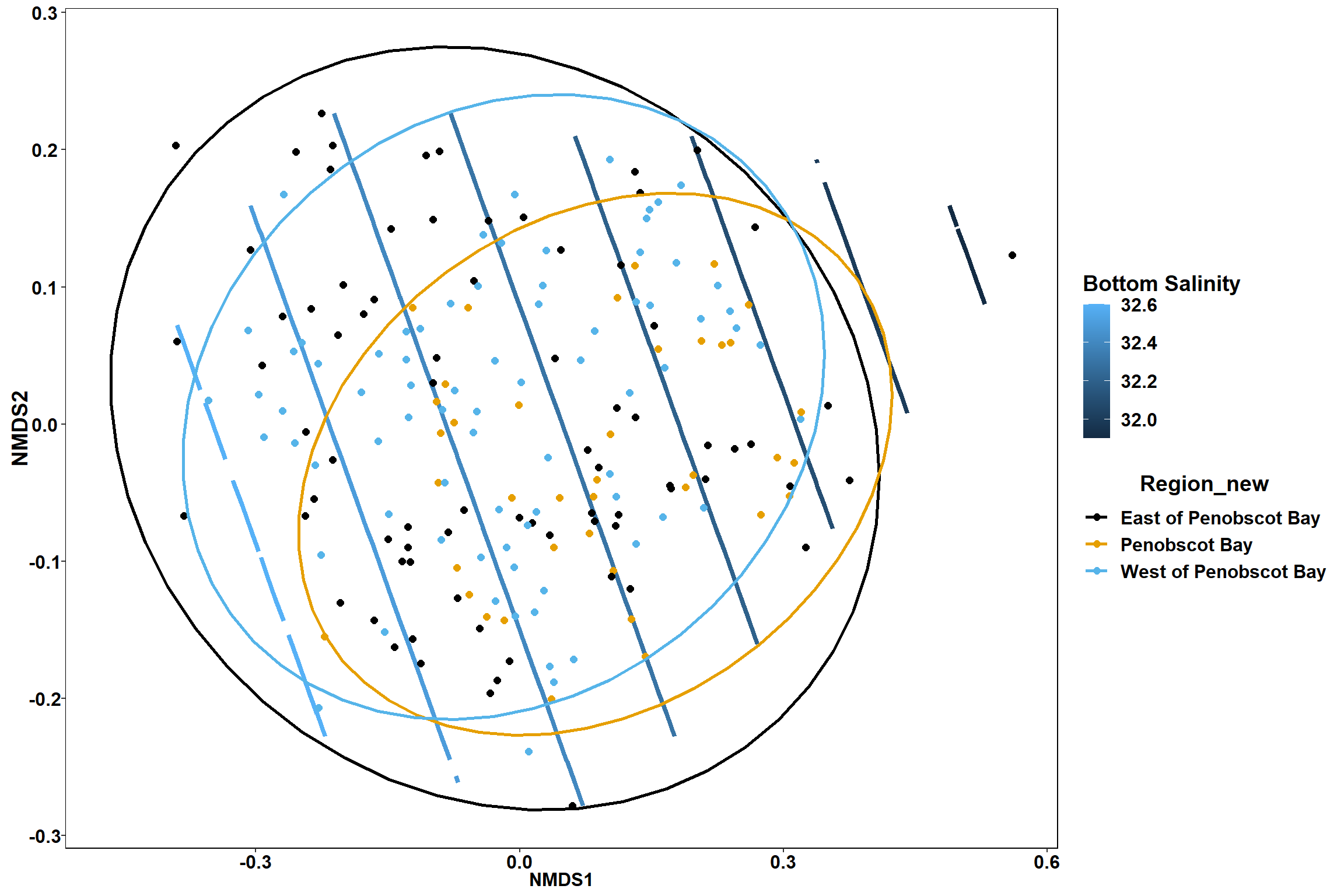
Surface salinity
surface_sal<-ordisurf(nmds, env$surface_sal)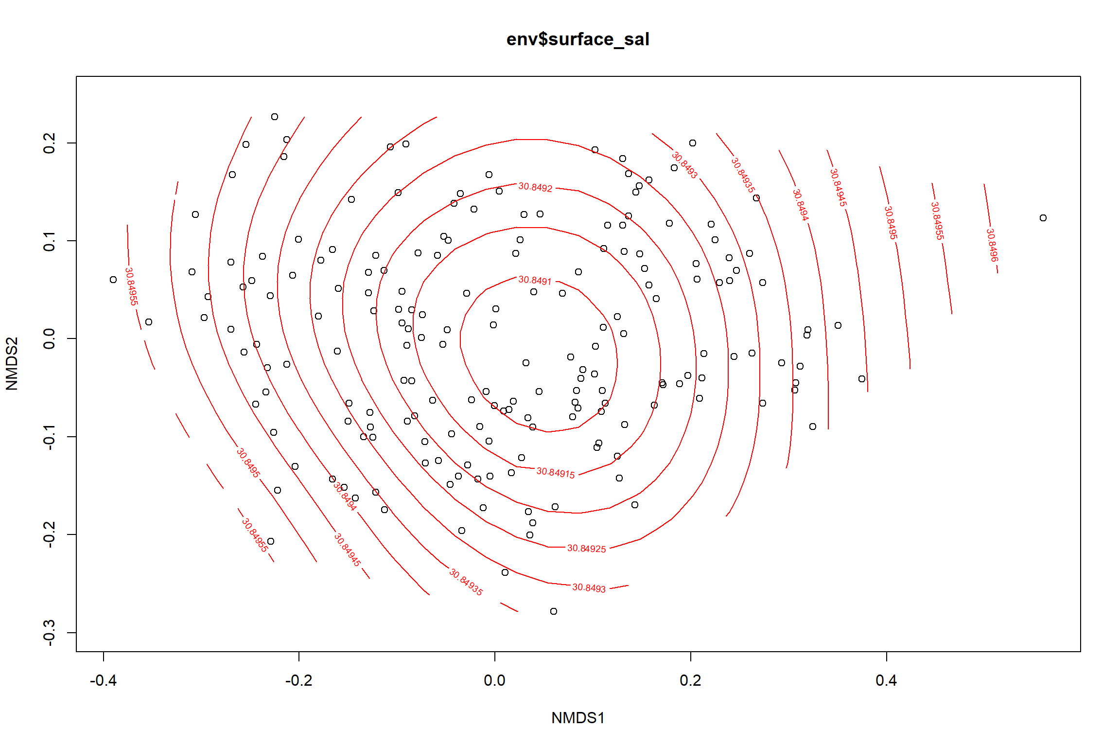
summary(surface_sal)##
## Family: gaussian
## Link function: identity
##
## Formula:
## y ~ s(x1, x2, k = 10, bs = "tp", fx = FALSE)
##
## Parametric coefficients:
## Estimate Std. Error t value Pr(>|t|)
## (Intercept) 30.8492 0.2342 131.7 <2e-16 ***
## ---
## Signif. codes: 0 '***' 0.001 '**' 0.01 '*' 0.05 '.' 0.1 ' ' 1
##
## Approximate significance of smooth terms:
## edf Ref.df F p-value
## s(x1,x2) 0.001547 9 0 0.627
##
## R-sq.(adj) = 2.6e-06 Deviance explained = 0.00108%
## -REML = 492.33 Scale est. = 10.425 n = 190ordi.grid <- surface_sal$grid #extracts the ordisurf object
#str(ordi.grid) #it's a list though - cannot be plotted as is
ordi.mite <- expand.grid(x = ordi.grid$x, y = ordi.grid$y) #get x and ys
ordi.mite$z <- as.vector(ordi.grid$z) #unravel the matrix for the z scores
contour.vals <- data.frame(na.omit(ordi.mite)) #gets rid of the nas
p <- ggplot()+
stat_contour(data = contour.vals, aes(x, y, z=z, color = ..level..),position="identity",size=1.5)+
labs(x = "NMDS1", y = "NMDS2", color="Surface Salinity")+
new_scale_color()+
geom_point(data = data.scores, aes(NMDS1, NMDS2, color=Year_groups, shape=Region_new), size = 3 )+ scale_color_colorblind()
p1 <- ggplot()+
stat_contour(data = contour.vals, aes(x, y, z=z, color = ..level..),position="identity",size=1.5)+
labs(x = "NMDS1", y = "NMDS2", color="Surface Salinity")+
new_scale_color()+
geom_point(data = data.scores, aes(NMDS1, NMDS2, color=Year_groups), size = 2 )+stat_ellipse(data=data.scores, aes(x=NMDS1, y=NMDS2, color=Year_groups),level = 0.95,size=1)+
scale_color_colorblind()
p2 <- ggplot()+
stat_contour(data = contour.vals, aes(x, y, z=z, color = ..level..),position="identity",size=1.5)+
labs(x = "NMDS1", y = "NMDS2", color="Surface Salinity")+
new_scale_color()+
geom_point(data = data.scores, aes(NMDS1, NMDS2, color=Region_new), size = 2 )+stat_ellipse(data=data.scores, aes(x=NMDS1, y=NMDS2, color=Region_new),level = 0.95,size=1)+
scale_color_colorblind()
p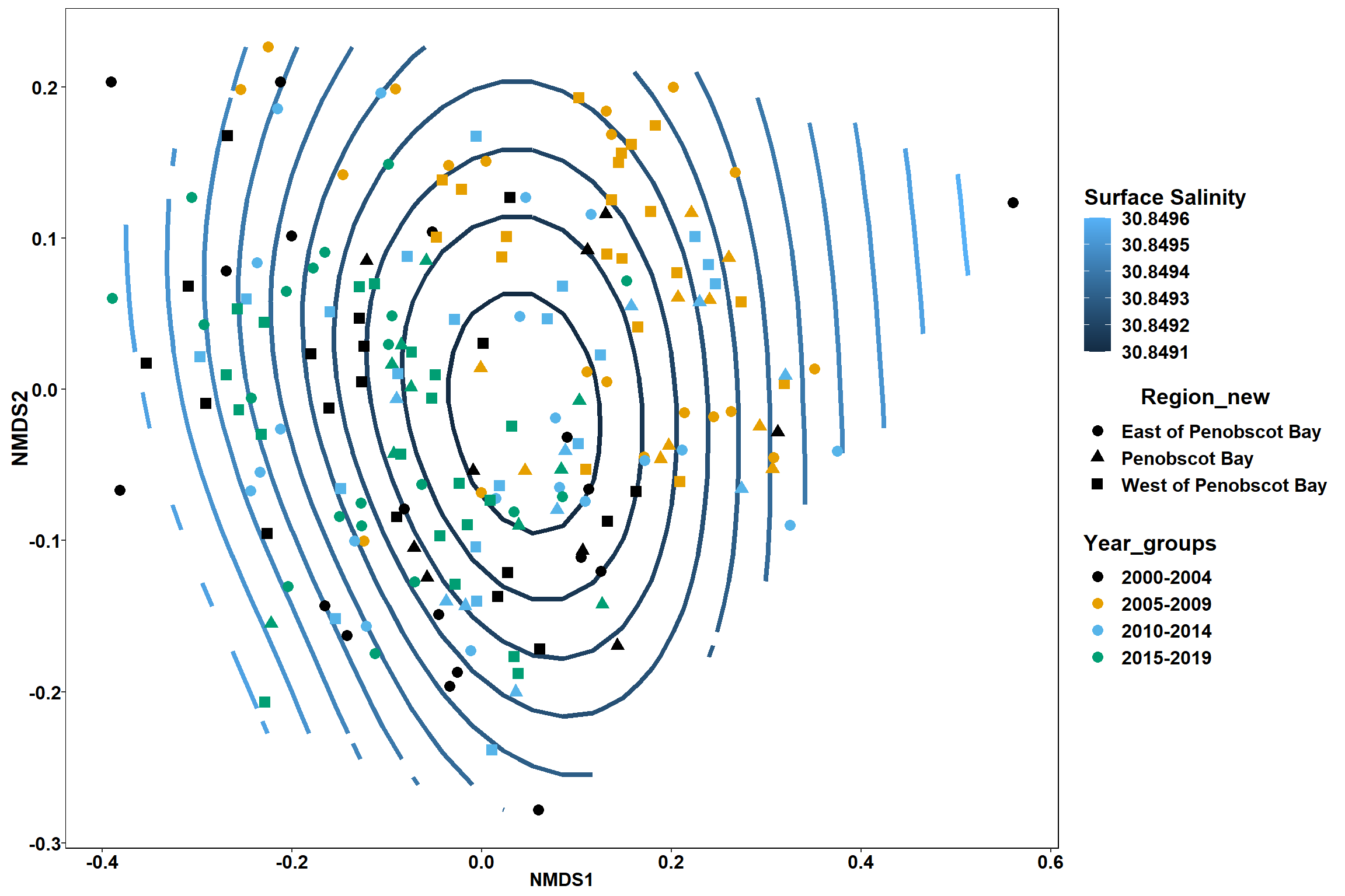
p1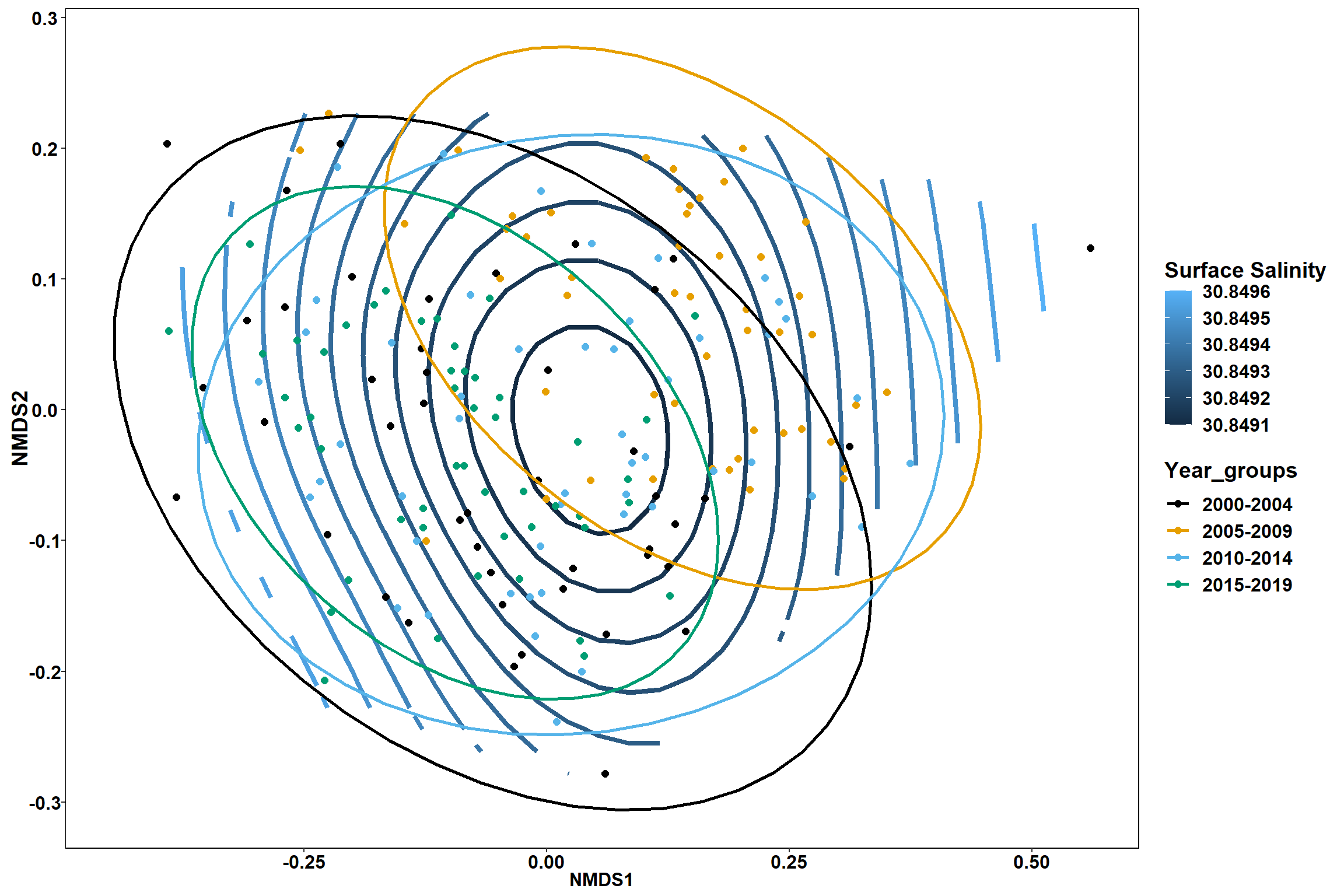
p2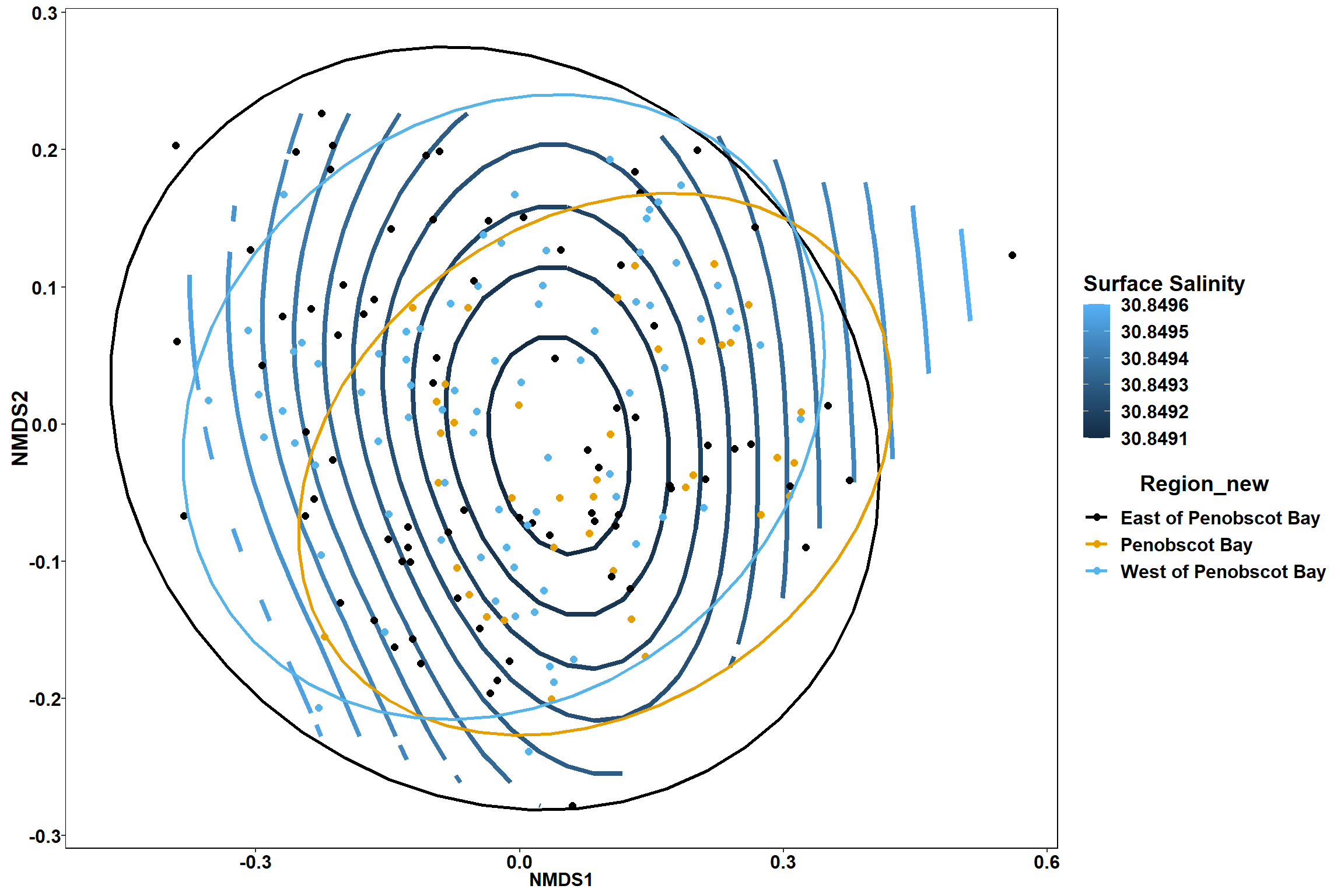
start latitude
start_lat<-ordisurf(nmds, env$start_lat)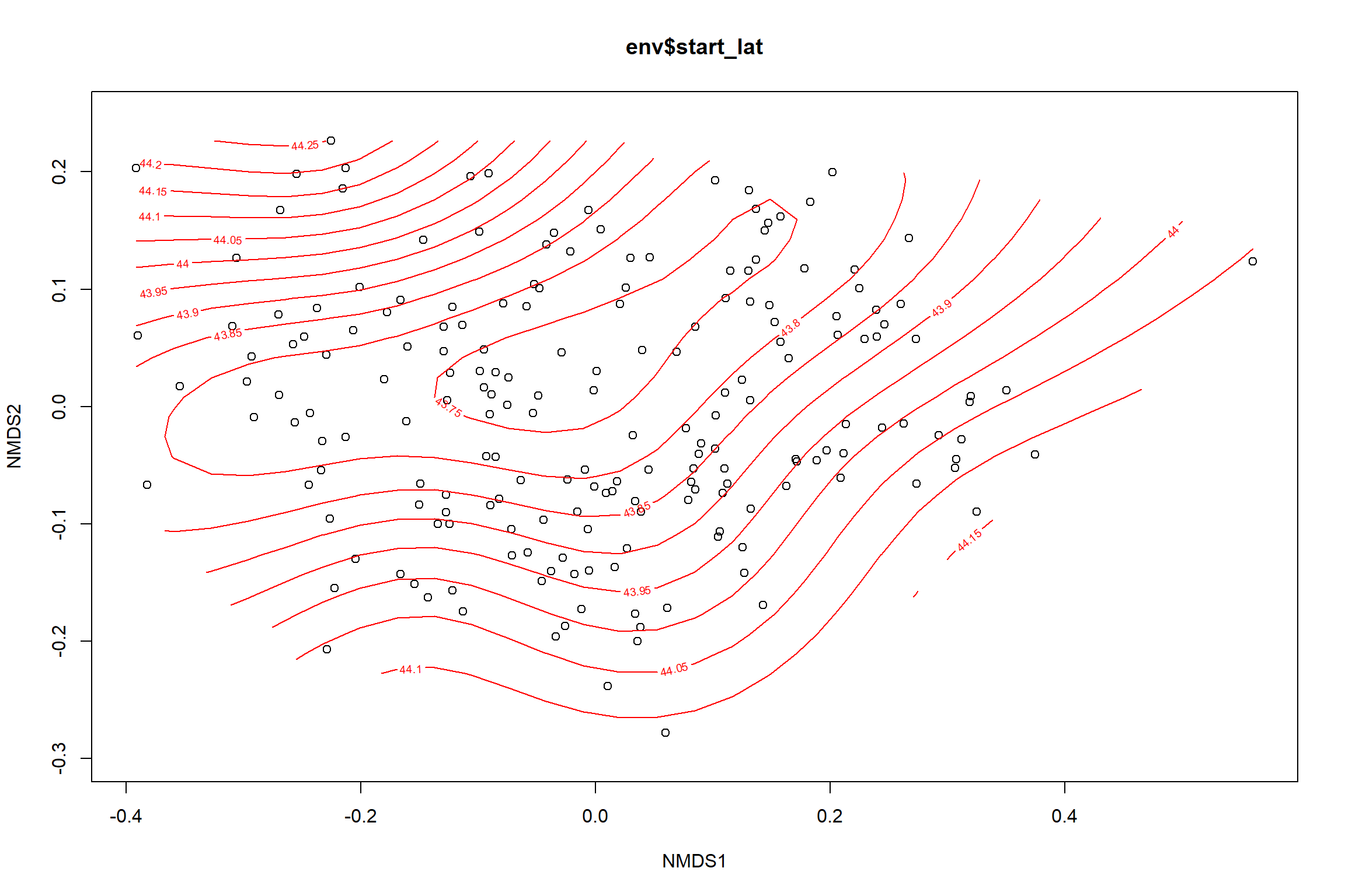
summary(start_lat)##
## Family: gaussian
## Link function: identity
##
## Formula:
## y ~ s(x1, x2, k = 10, bs = "tp", fx = FALSE)
##
## Parametric coefficients:
## Estimate Std. Error t value Pr(>|t|)
## (Intercept) 43.8750 0.0294 1493 <2e-16 ***
## ---
## Signif. codes: 0 '***' 0.001 '**' 0.01 '*' 0.05 '.' 0.1 ' ' 1
##
## Approximate significance of smooth terms:
## edf Ref.df F p-value
## s(x1,x2) 5.385 9 2.312 0.000787 ***
## ---
## Signif. codes: 0 '***' 0.001 '**' 0.01 '*' 0.05 '.' 0.1 ' ' 1
##
## R-sq.(adj) = 0.0969 Deviance explained = 12.2%
## -REML = 111.2 Scale est. = 0.16851 n = 195ordi.grid <- start_lat$grid #extracts the ordisurf object
#str(ordi.grid) #it's a list though - cannot be plotted as is
ordi.mite <- expand.grid(x = ordi.grid$x, y = ordi.grid$y) #get x and ys
ordi.mite$z <- as.vector(ordi.grid$z) #unravel the matrix for the z scores
contour.vals <- data.frame(na.omit(ordi.mite)) #gets rid of the nas
p <- ggplot()+
stat_contour(data = contour.vals, aes(x, y, z=z, color = ..level..),position="identity",size=1.5)+
labs(x = "NMDS1", y = "NMDS2", color="Latitude")+
new_scale_color()+
geom_point(data = data.scores, aes(NMDS1, NMDS2, color=Year_groups, shape=Region_new), size = 3 )+ scale_color_colorblind()
p1 <- ggplot()+
stat_contour(data = contour.vals, aes(x, y, z=z, color = ..level..),position="identity",size=1.5)+
labs(x = "NMDS1", y = "NMDS2", color="Latitude")+
new_scale_color()+
geom_point(data = data.scores, aes(NMDS1, NMDS2, color=Year_groups), size = 2 )+ stat_ellipse(data=data.scores, aes(x=NMDS1, y=NMDS2, color=Year_groups),level = 0.95,size=1)+
scale_color_colorblind()
p2 <- ggplot()+
stat_contour(data = contour.vals, aes(x, y, z=z, color = ..level..),position="identity",size=1.5)+
labs(x = "NMDS1", y = "NMDS2", color="Latitude")+
new_scale_color()+
geom_point(data = data.scores, aes(NMDS1, NMDS2, color=Region_new), size = 2 )+ stat_ellipse(data=data.scores, aes(x=NMDS1, y=NMDS2, color=Region_new),level = 0.95,size=1)+
scale_color_colorblind()
p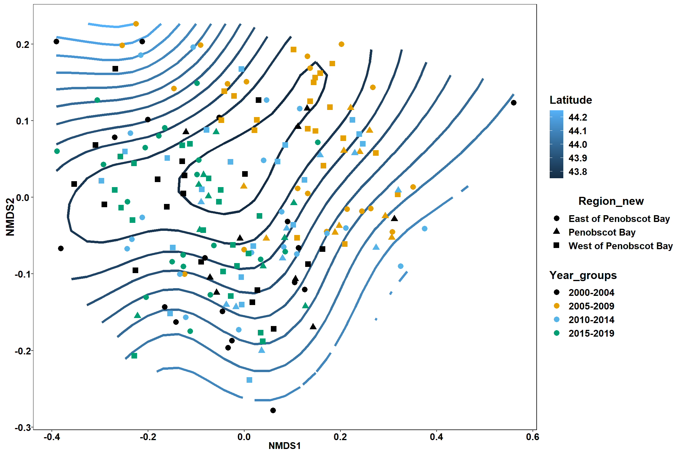
p1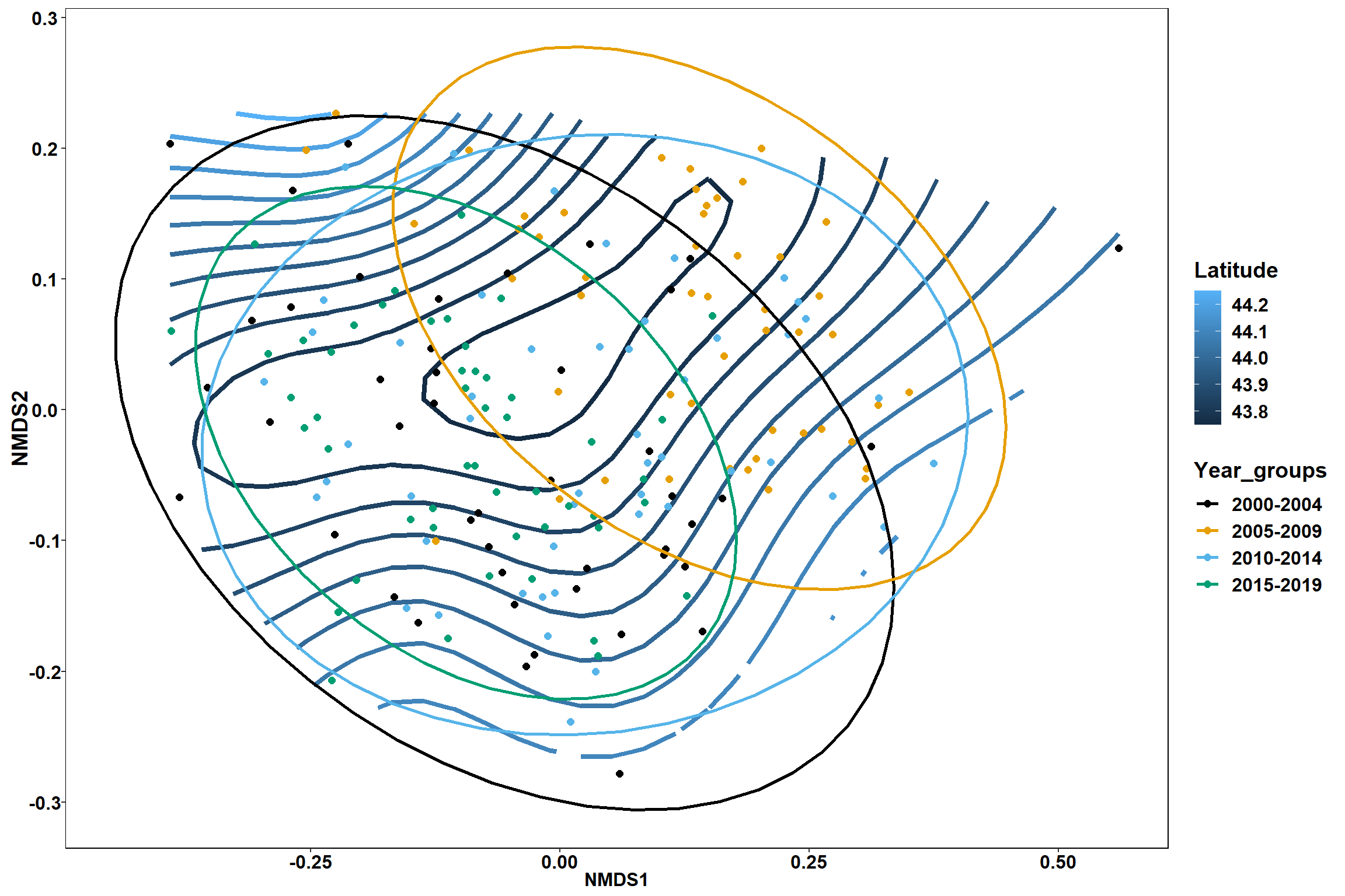
p2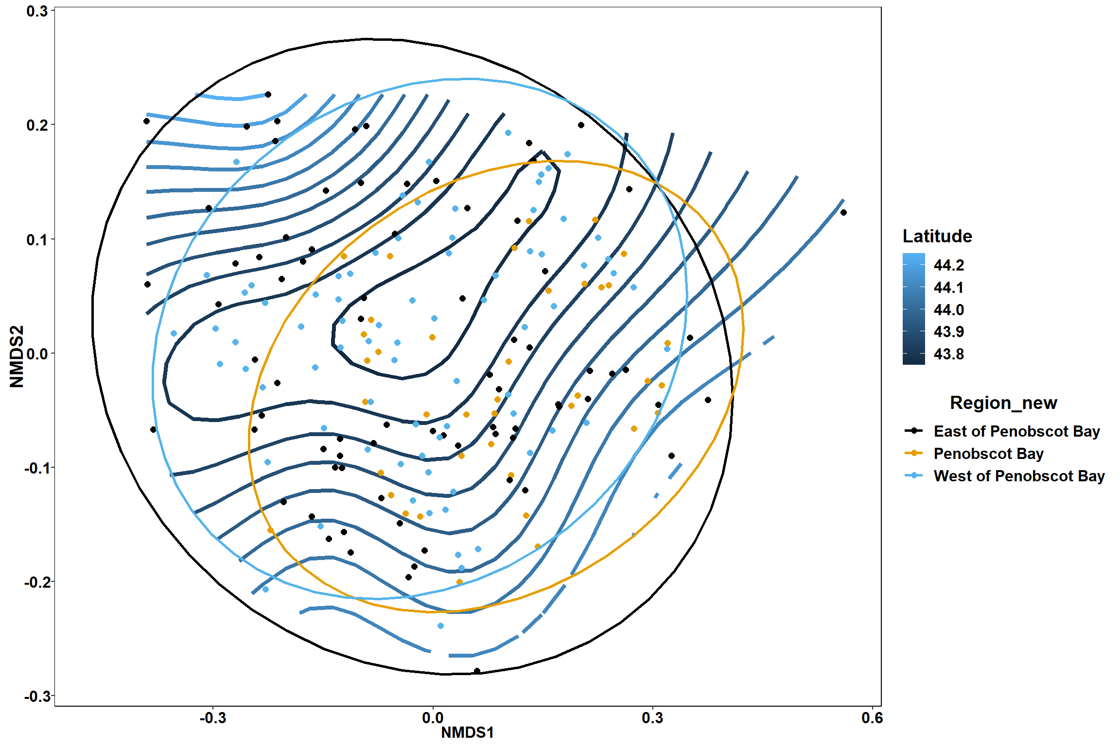
start longitude
start_long<-ordisurf(nmds, env$start_long)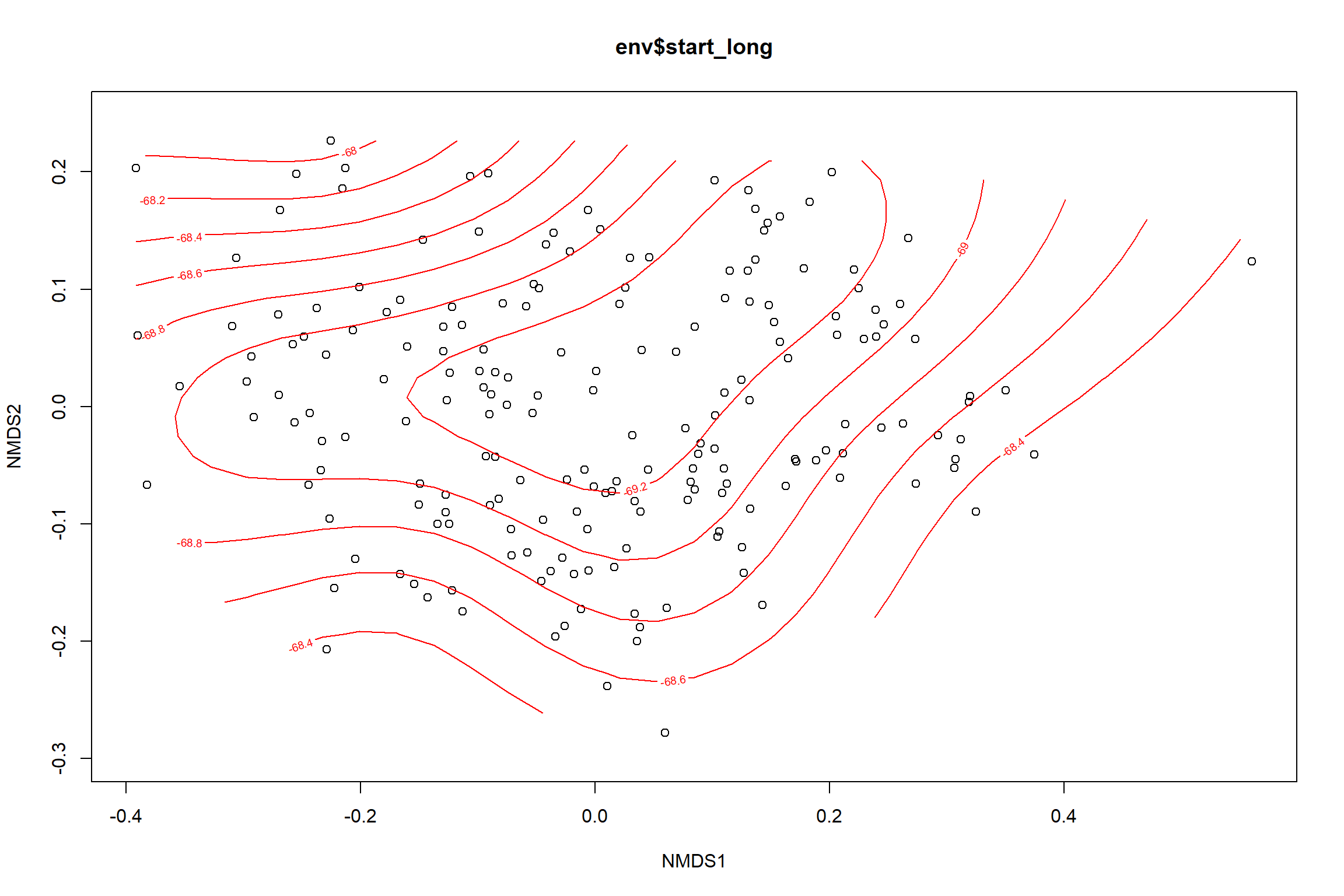
summary(start_long)##
## Family: gaussian
## Link function: identity
##
## Formula:
## y ~ s(x1, x2, k = 10, bs = "tp", fx = FALSE)
##
## Parametric coefficients:
## Estimate Std. Error t value Pr(>|t|)
## (Intercept) -68.97337 0.06958 -991.3 <2e-16 ***
## ---
## Signif. codes: 0 '***' 0.001 '**' 0.01 '*' 0.05 '.' 0.1 ' ' 1
##
## Approximate significance of smooth terms:
## edf Ref.df F p-value
## s(x1,x2) 5.552 9 2.623 0.000294 ***
## ---
## Signif. codes: 0 '***' 0.001 '**' 0.01 '*' 0.05 '.' 0.1 ' ' 1
##
## R-sq.(adj) = 0.108 Deviance explained = 13.4%
## -REML = 278.78 Scale est. = 0.94399 n = 195ordi.grid <- start_long$grid #extracts the ordisurf object
#str(ordi.grid) #it's a list though - cannot be plotted as is
ordi.mite <- expand.grid(x = ordi.grid$x, y = ordi.grid$y) #get x and ys
ordi.mite$z <- as.vector(ordi.grid$z) #unravel the matrix for the z scores
contour.vals <- data.frame(na.omit(ordi.mite)) #gets rid of the nas
p <- ggplot()+
stat_contour(data = contour.vals, aes(x, y, z=z, color = ..level..),position="identity",size=1.5)+
labs(x = "NMDS1", y = "NMDS2", color="Longitude")+
new_scale_color()+
geom_point(data = data.scores, aes(NMDS1, NMDS2, color=Year_groups, shape=Region_new), size = 3 )+ scale_color_colorblind()
p1 <- ggplot()+
stat_contour(data = contour.vals, aes(x, y, z=z, color = ..level..),position="identity",size=1.5)+
labs(x = "NMDS1", y = "NMDS2", color="Longitude")+
new_scale_color()+
geom_point(data = data.scores, aes(NMDS1, NMDS2, color=Year_groups), size = 2 )+stat_ellipse(data=data.scores, aes(x=NMDS1, y=NMDS2, color=Year_groups),level = 0.95,size=1)+
scale_color_colorblind()
p2 <- ggplot()+
stat_contour(data = contour.vals, aes(x, y, z=z, color = ..level..),position="identity",size=1.5)+
labs(x = "NMDS1", y = "NMDS2", color="Longitude")+
new_scale_color()+
geom_point(data = data.scores, aes(NMDS1, NMDS2, color=Region_new), size = 2 )+stat_ellipse(data=data.scores, aes(x=NMDS1, y=NMDS2, color=Region_new),level = 0.95,size=1)+
scale_color_colorblind()
p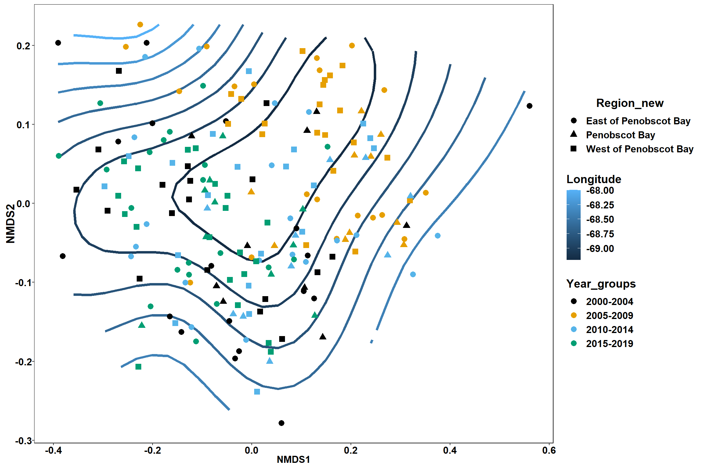
p1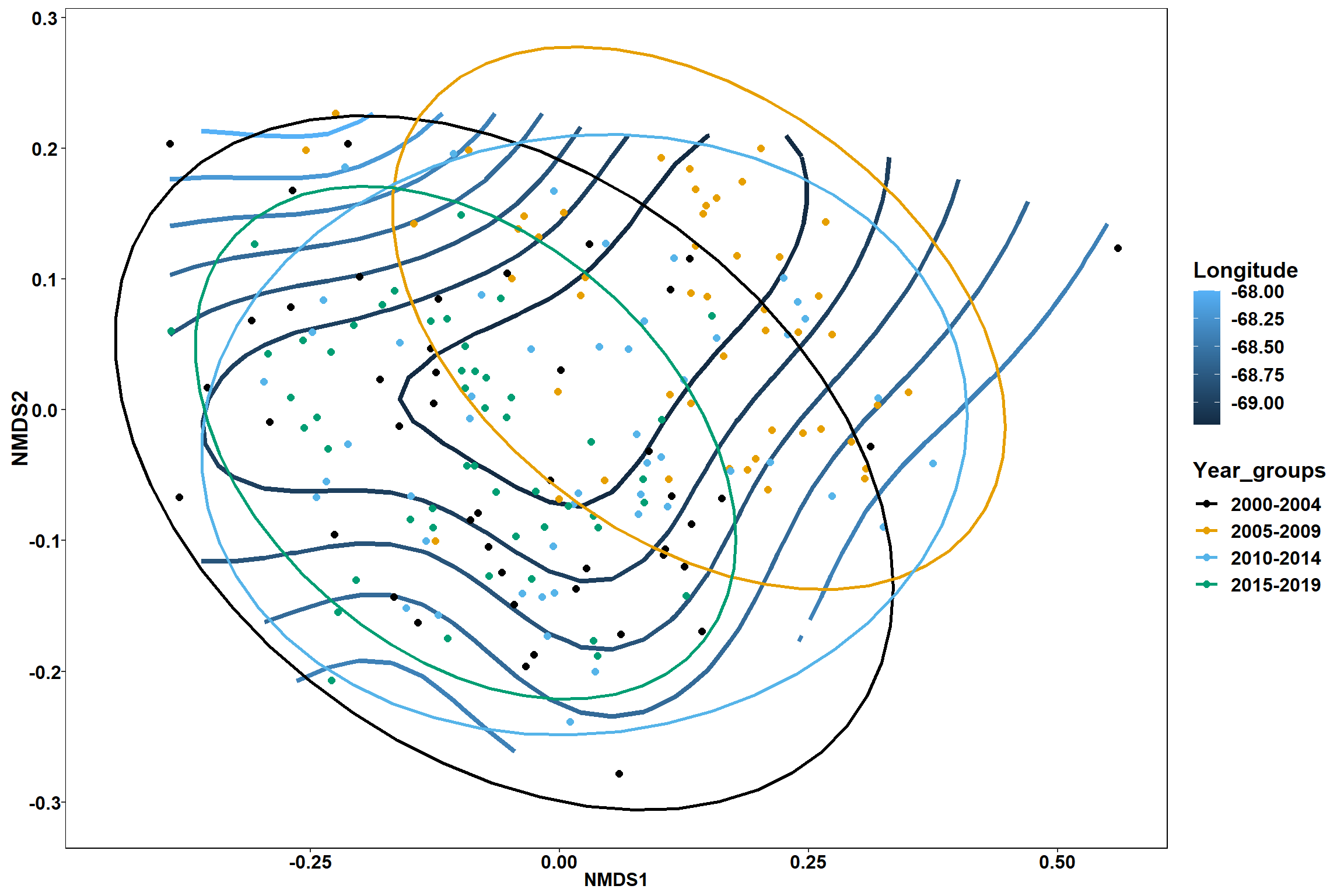
p2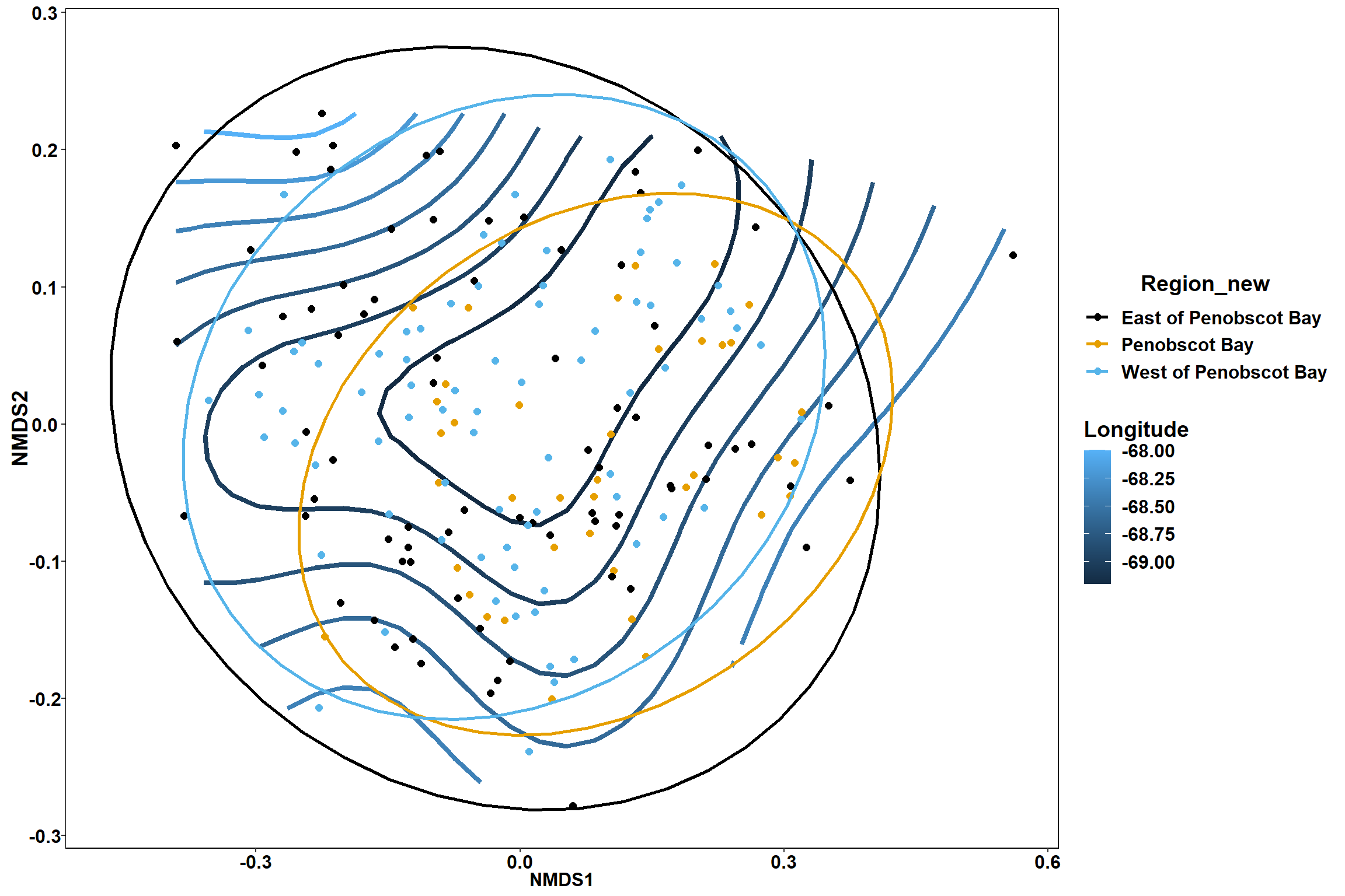
start depth
start_depth<-ordisurf(nmds, env$start_depth)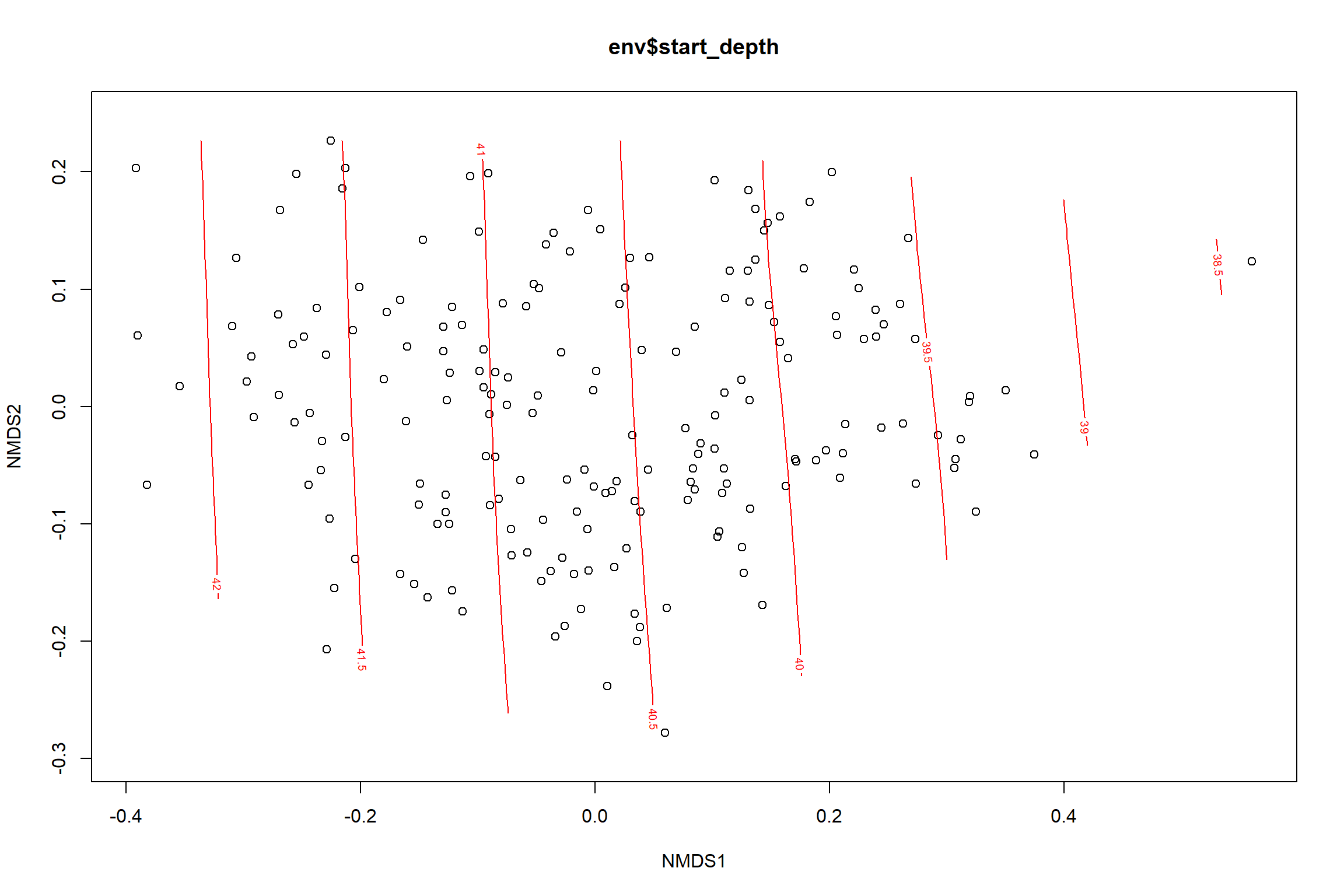
summary(start_depth)##
## Family: gaussian
## Link function: identity
##
## Formula:
## y ~ s(x1, x2, k = 10, bs = "tp", fx = FALSE)
##
## Parametric coefficients:
## Estimate Std. Error t value Pr(>|t|)
## (Intercept) 40.6472 0.3171 128.2 <2e-16 ***
## ---
## Signif. codes: 0 '***' 0.001 '**' 0.01 '*' 0.05 '.' 0.1 ' ' 1
##
## Approximate significance of smooth terms:
## edf Ref.df F p-value
## s(x1,x2) 1.627 9 0.744 0.015 *
## ---
## Signif. codes: 0 '***' 0.001 '**' 0.01 '*' 0.05 '.' 0.1 ' ' 1
##
## R-sq.(adj) = 0.0334 Deviance explained = 4.15%
## -REML = 568.05 Scale est. = 19.602 n = 195ordi.grid <- start_depth$grid #extracts the ordisurf object
#str(ordi.grid) #it's a list though - cannot be plotted as is
ordi.mite <- expand.grid(x = ordi.grid$x, y = ordi.grid$y) #get x and ys
ordi.mite$z <- as.vector(ordi.grid$z) #unravel the matrix for the z scores
contour.vals <- data.frame(na.omit(ordi.mite)) #gets rid of the nas
p <- ggplot()+
stat_contour(data = contour.vals, aes(x, y, z=z, color = ..level..),position="identity",size=1.5)+
labs(x = "NMDS1", y = "NMDS2", color="Depth")+
new_scale_color()+
geom_point(data = data.scores, aes(NMDS1, NMDS2, color=Year_groups, shape=Region_new), size = 3 )+ scale_color_colorblind()
p1 <- ggplot()+
stat_contour(data = contour.vals, aes(x, y, z=z, color = ..level..),position="identity",size=1.5)+
labs(x = "NMDS1", y = "NMDS2", color="Depth")+
new_scale_color()+
geom_point(data = data.scores, aes(NMDS1, NMDS2, color=Year_groups), size = 2 )+stat_ellipse(data=data.scores, aes(x=NMDS1, y=NMDS2, color=Year_groups),level = 0.95,size=1)+
scale_color_colorblind()
p2 <- ggplot()+
stat_contour(data = contour.vals, aes(x, y, z=z, color = ..level..),position="identity",size=1.5)+
labs(x = "NMDS1", y = "NMDS2", color="Depth")+
new_scale_color()+
geom_point(data = data.scores, aes(NMDS1, NMDS2, color=Region_new), size = 2 )+stat_ellipse(data=data.scores, aes(x=NMDS1, y=NMDS2, color=Region_new),level = 0.95,size=1)+
scale_color_colorblind()
p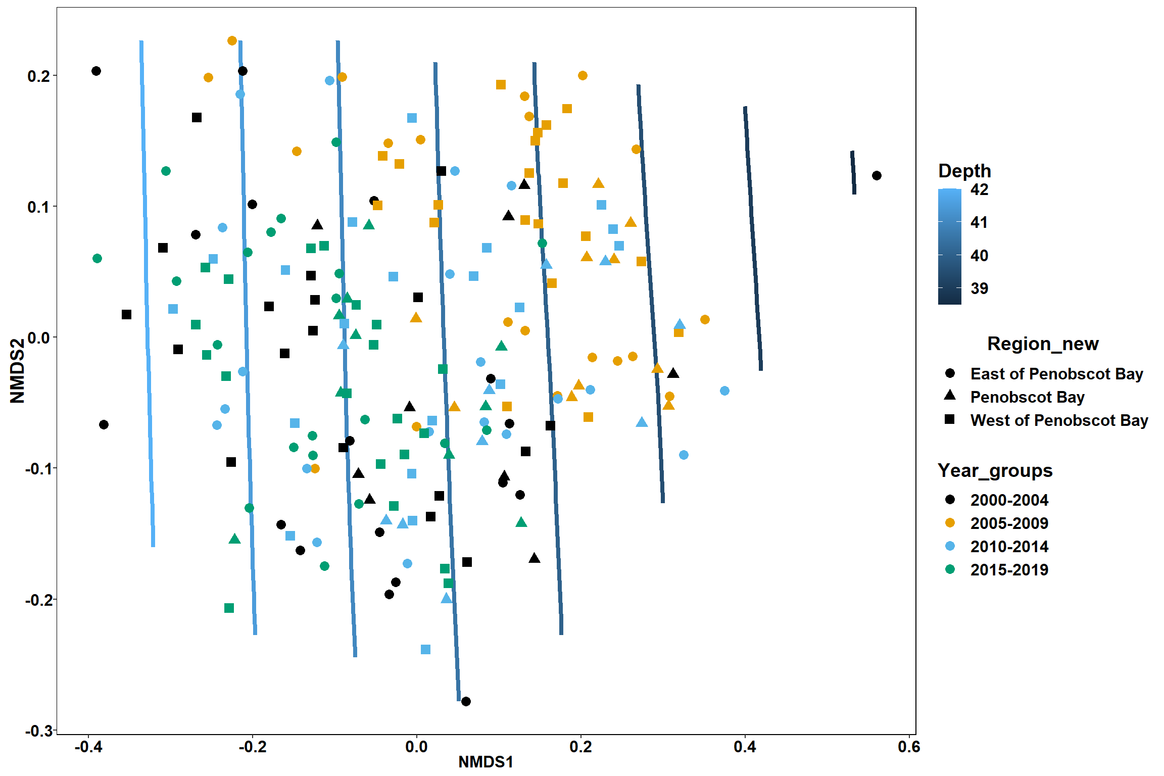
p1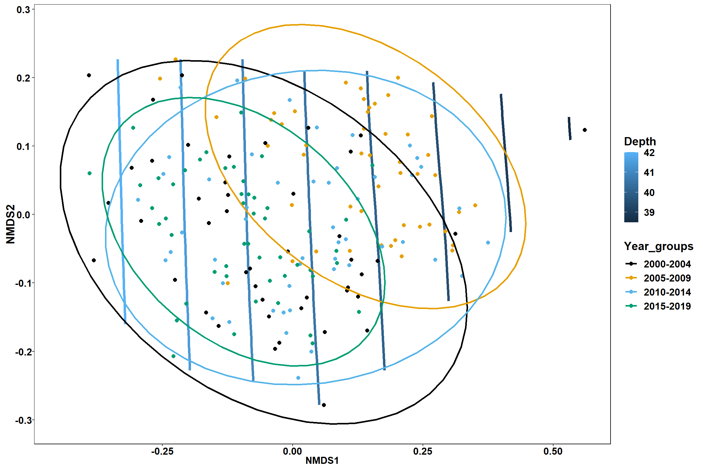
p2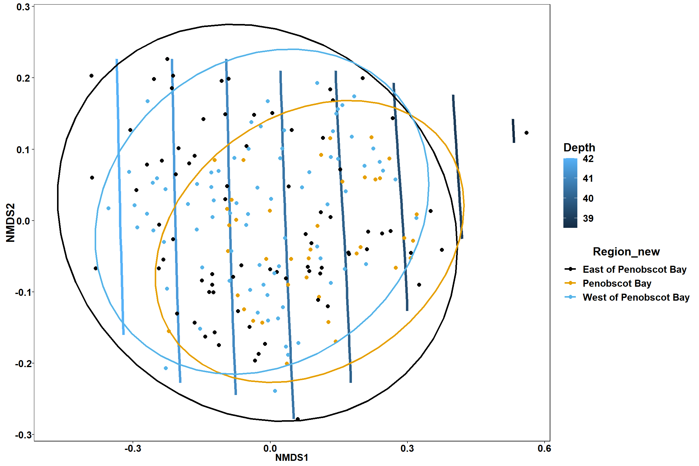
Top 50 Species Abundance
NMDS
#load in data
trawl_data_arrange<-read.csv(here("Data/species_abundance_matrix.csv"))[-1]

trawl_data<-read.csv(here("Data/MaineDMR_Trawl_Survey_Tow_Data_2021-05-14.csv"))

all_Data<-group_by(trawl_data, Season, Year, Region)%>%
  filter(Year<2020)%>%
  summarise(start_lat=mean(Start_Latitude),start_long=mean(Start_Longitude),end_lat=mean(End_Latitude), end_long=mean(End_Longitude),start_depth=mean(Start_Depth_fathoms, na.rm=TRUE), end_depth=mean(End_Depth_fathoms, na.rm=TRUE), bottom_temp=mean(Bottom_WaterTemp_DegC, na.rm=TRUE), bottom_sal=mean(Bottom_Salinity, na.rm=TRUE),surface_temp=mean(Surface_WaterTemp_DegC, na.rm=TRUE), surface_sal=mean(Surface_Salinity, na.rm=TRUE))%>%
  full_join(trawl_data_arrange)%>%
  ungroup()

com<-select(all_Data, 14:63)

com<-vegdist(com, method="bray")

#convert com to a matrix
m_com = as.matrix(com)

set.seed(123)
nmds = metaMDS(m_com,k=2, distance = "bray", trymax = 200)
## Run 0 stress 0.1621597
## Run 1 stress 0.1790884
## Run 2 stress 0.1624906
## ... Procrustes: rmse 0.009948471 max resid 0.1360388
## Run 3 stress 0.166605
## Run 4 stress 0.1659038
## Run 5 stress 0.1784512
## Run 6 stress 0.1666044
## Run 7 stress 0.175383
## Run 8 stress 0.1829157
## Run 9 stress 0.1659039
## Run 10 stress 0.1662477
## Run 11 stress 0.1621603
## ... Procrustes: rmse 0.0002541615 max resid 0.003157041
## ... Similar to previous best
## Run 12 stress 0.175406
## Run 13 stress 0.165904
## Run 14 stress 0.1621599
## ... Procrustes: rmse 0.0001949799 max resid 0.002529041
## ... Similar to previous best
## Run 15 stress 0.1755351
## Run 16 stress 0.1697831
## Run 17 stress 0.1699906
## Run 18 stress 0.1662485
## Run 19 stress 0.1666052
## Run 20 stress 0.1699906
## *** Solution reachednmds##
## Call:
## metaMDS(comm = m_com, distance = "bray", k = 2, trymax = 200)
##
## global Multidimensional Scaling using monoMDS
##
## Data: m_com
## Distance: user supplied
##
## Dimensions: 2
## Stress: 0.1621597
## Stress type 1, weak ties
## Two convergent solutions found after 20 tries
## Scaling: centring, PC rotation
## Species: scores missingEnvfit
env<-select(all_Data, start_lat, start_long, end_lat, end_long,start_depth, end_depth, bottom_temp, bottom_sal, surface_temp, surface_sal)

en<-envfit(nmds, env, permutations=999, na.rm=TRUE)
en
##
## ***VECTORS
##
## NMDS1 NMDS2 r2 Pr(>r)
## start_lat 0.34812 0.93745 0.1120 0.001 ***
## start_long 0.16650 0.98604 0.0953 0.001 ***
## end_lat 0.34992 0.93678 0.1113 0.001 ***
## end_long 0.16648 0.98605 0.0954 0.001 ***
## start_depth -0.12190 -0.99254 0.0357 0.032 *
## end_depth -0.09046 -0.99590 0.0246 0.096 .
## bottom_temp -0.14219 -0.98984 0.1301 0.001 ***
## bottom_sal -0.43031 -0.90268 0.1064 0.001 ***
## surface_temp -0.20442 -0.97888 0.2951 0.001 ***
## surface_sal 0.24819 -0.96871 0.0002 0.986
## ---
## Signif. codes: 0 '***' 0.001 '**' 0.01 '*' 0.05 '.' 0.1 ' ' 1
## Permutation: free
## Number of permutations: 999
##
## 5 observations deleted due to missingnessplot(nmds)
plot(en)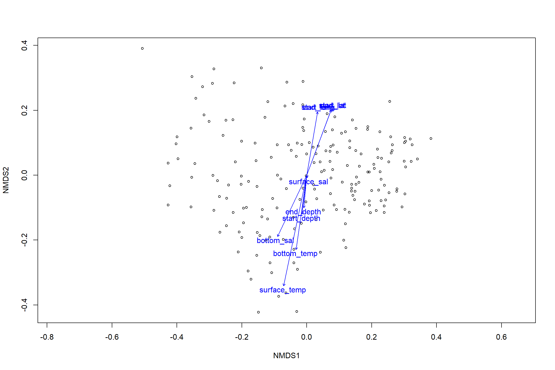
en_coord_cont = as.data.frame(scores(en, "vectors")) * ordiArrowMul(en)
en_coord_cat = as.data.frame(scores(en, "factors")) * ordiArrowMul(en)

#extract NMDS scores for ggplot
data.scores = as.data.frame(scores(nmds))
#add columns to data frame
data.scores$Region = all_Data$Region
data.scores$Year = all_Data$Year
data.scores$Season= all_Data$Season
data.scores$Year_groups= all_Data$YEAR_GROUPS
data.scores$Year_decades= all_Data$YEAR_DECADES
data.scores$Region_new=all_Data$REGION_NEW
data.scores$Region_year=all_Data$REGION_YEAR
data.scores$Season_year=all_Data$SEASON_YEAR

p<- ggplot()+
     geom_point(data = data.scores, aes(x = NMDS1, y = NMDS2, color=Year_groups, shape=Region_new), size = 4) +
  scale_color_colorblind()+
        geom_segment(data=en_coord_cont, aes(x = 0, y = 0, xend = NMDS1, yend = NMDS2), size =1.5, alpha = 0.5)+
   geom_text(data = en_coord_cont, aes(x = NMDS1, y = NMDS2), size=5,
       fontface = "bold", label = row.names(en_coord_cont))+
    theme(axis.title = element_text(size = 16, face = "bold"),
       panel.background = element_blank(), panel.border = element_rect(fill = NA),
       axis.ticks = element_blank(), axis.text = element_blank(), legend.key = element_blank(),
       legend.title = element_text(size = 16, face = "bold"),
       legend.text = element_text(size = 16))


p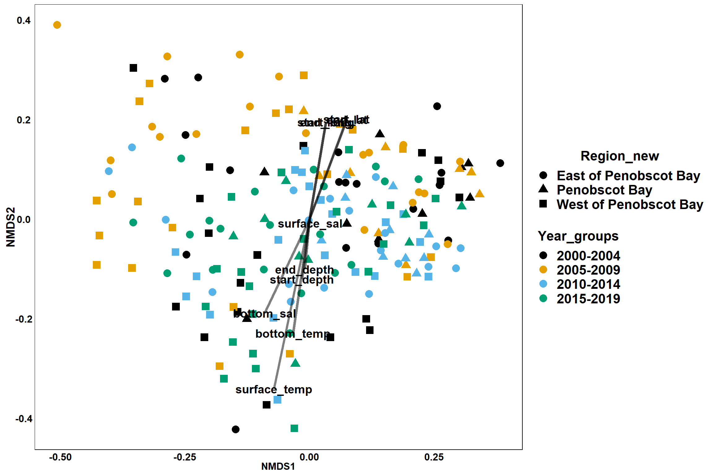
Region groups
p_region<- ggplot()+
     geom_point(data = data.scores, aes(x = NMDS1, y = NMDS2, color=Region_new), size = 4) +
  scale_color_colorblind()+
        geom_segment(data=en_coord_cont, aes(x = 0, y = 0, xend = NMDS1, yend = NMDS2), size =1.5, alpha = 0.5)+
   geom_text(data = en_coord_cont, aes(x = NMDS1, y = NMDS2), size=5,
       fontface = "bold", label = row.names(en_coord_cont))+
  stat_ellipse(data=data.scores, aes(x=NMDS1, y=NMDS2, color=Region_new),level = 0.95,size=1)+
  theme(axis.title = element_text(size = 16, face = "bold"),
       panel.background = element_blank(), panel.border = element_rect(fill = NA),
       axis.ticks = element_blank(), axis.text = element_blank(), legend.key = element_blank(),
       legend.title = element_text(size = 16, face = "bold"),
       legend.text = element_text(size = 16))


p_region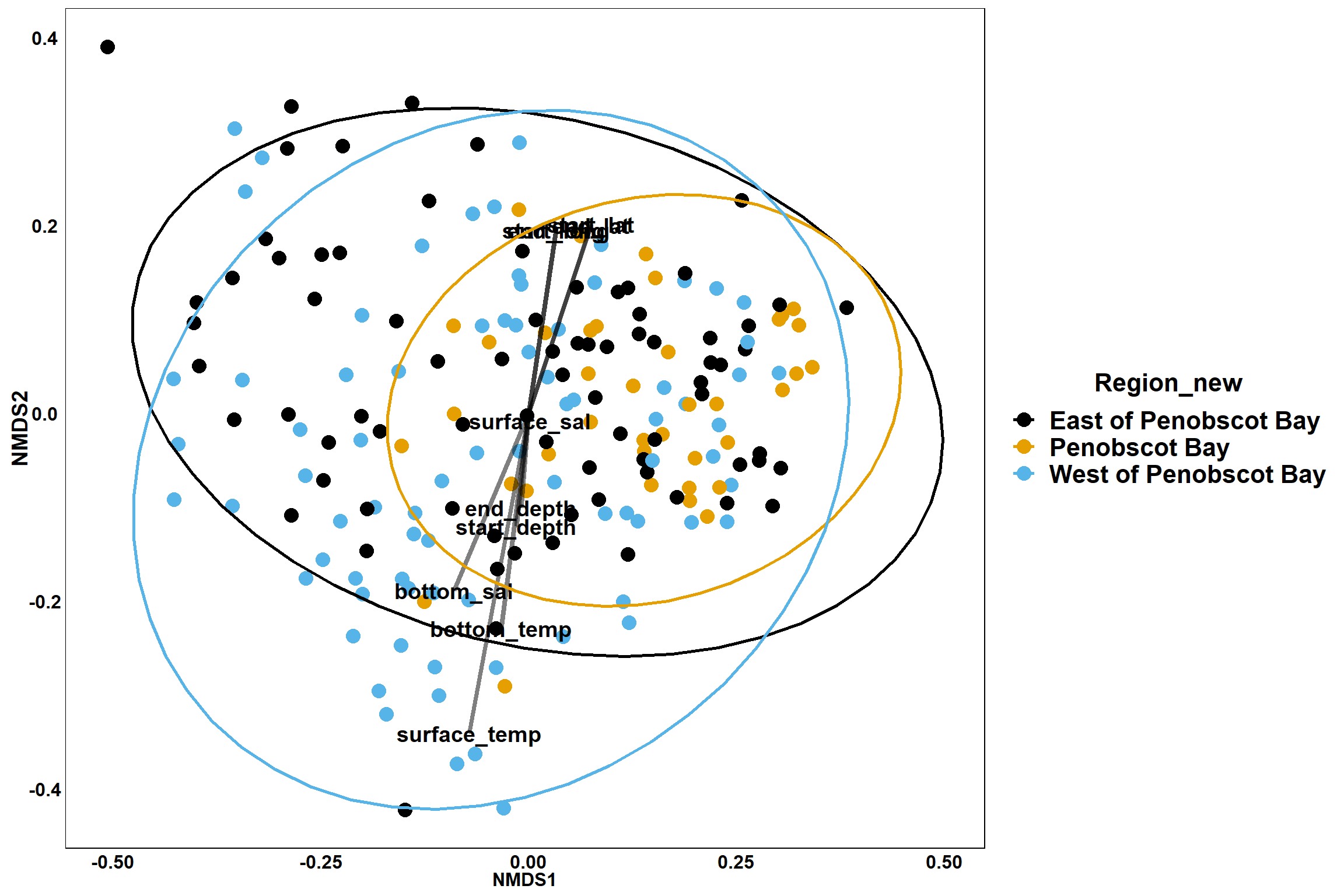
Year groups
p_year<- ggplot()+
     geom_point(data = data.scores, aes(x = NMDS1, y = NMDS2, color=Year_groups), size = 4) +
  scale_color_colorblind()+
        geom_segment(data=en_coord_cont, aes(x = 0, y = 0, xend = NMDS1, yend = NMDS2), size =1.5, alpha = 0.5)+
   geom_text(data = en_coord_cont, aes(x = NMDS1, y = NMDS2), size=5,
       fontface = "bold", label = row.names(en_coord_cont))+
  stat_ellipse(data=data.scores, aes(x=NMDS1, y=NMDS2, color=Year_groups),level = 0.95,size=1)+
  theme(axis.title = element_text(size = 16, face = "bold"),
       panel.background = element_blank(), panel.border = element_rect(fill = NA),
       axis.ticks = element_blank(), axis.text = element_blank(), legend.key = element_blank(),
       legend.title = element_text(size = 16, face = "bold"),
       legend.text = element_text(size = 16))

p_year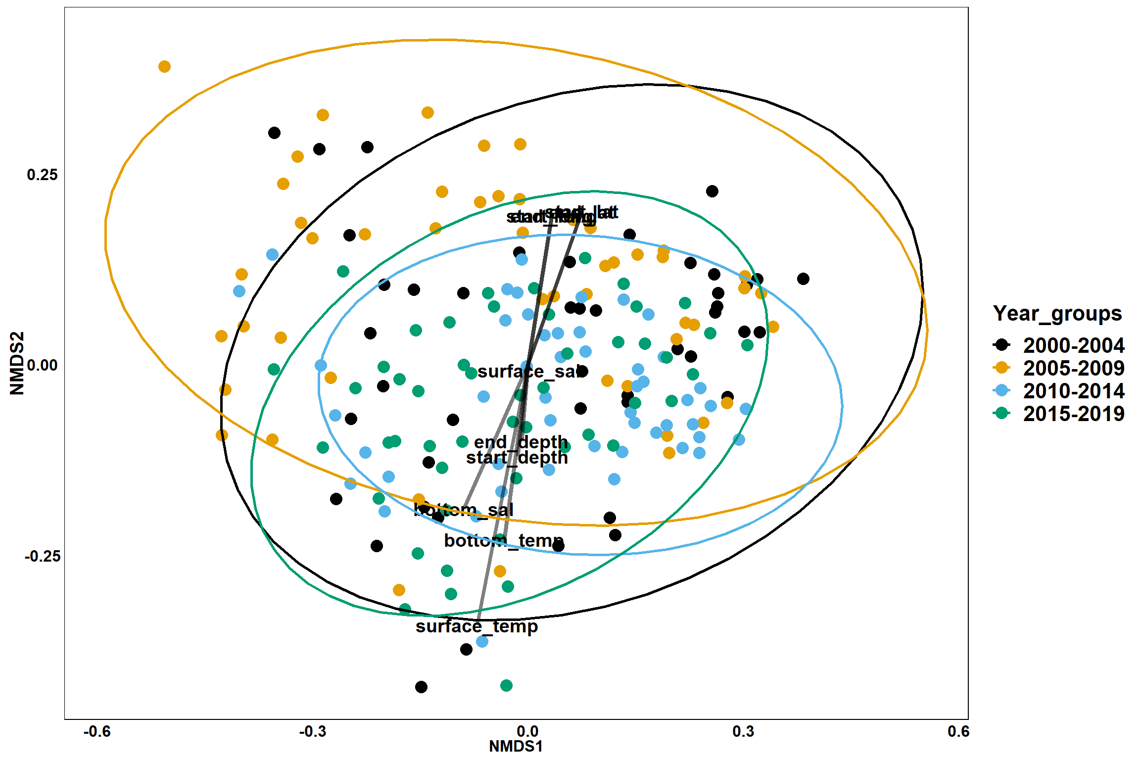
GAM contours for environmental effects
Bottom temperature
bottom_temp<-ordisurf(nmds, env$bottom_temp)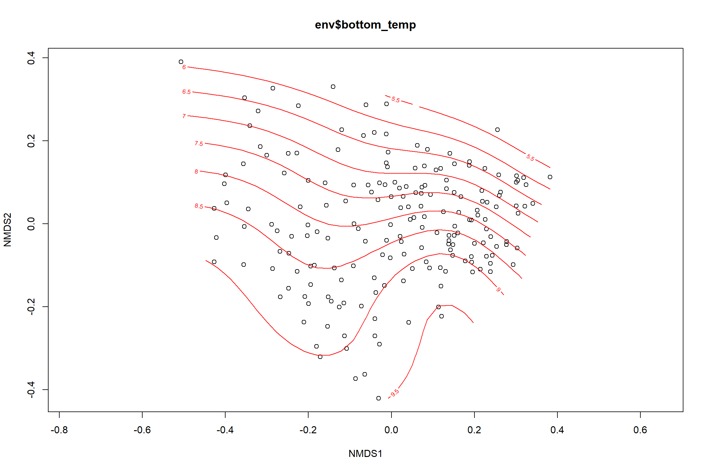
summary(bottom_temp)##
## Family: gaussian
## Link function: identity
##
## Formula:
## y ~ s(x1, x2, k = 10, bs = "tp", fx = FALSE)
##
## Parametric coefficients:
## Estimate Std. Error t value Pr(>|t|)
## (Intercept) 7.9053 0.1719 45.98 <2e-16 ***
## ---
## Signif. codes: 0 '***' 0.001 '**' 0.01 '*' 0.05 '.' 0.1 ' ' 1
##
## Approximate significance of smooth terms:
## edf Ref.df F p-value
## s(x1,x2) 5.473 9 4.253 6.89e-07 ***
## ---
## Signif. codes: 0 '***' 0.001 '**' 0.01 '*' 0.05 '.' 0.1 ' ' 1
##
## R-sq.(adj) = 0.168 Deviance explained = 19.2%
## -REML = 439.82 Scale est. = 5.6159 n = 190ordi.grid <- bottom_temp$grid #extracts the ordisurf object
#str(ordi.grid) #it's a list though - cannot be plotted as is
ordi.mite <- expand.grid(x = ordi.grid$x, y = ordi.grid$y) #get x and ys
ordi.mite$z <- as.vector(ordi.grid$z) #unravel the matrix for the z scores
contour.vals <- data.frame(na.omit(ordi.mite)) #gets rid of the nas
p <- ggplot()+
stat_contour(data = contour.vals, aes(x, y, z=z, color = ..level..),position="identity",size=1.5)+
labs(x = "NMDS1", y = "NMDS2", color="Bottom Temperature")+
new_scale_color()+
geom_point(data = data.scores, aes(NMDS1, NMDS2, color=Year_groups, shape=Region_new), size = 3 )+ scale_color_colorblind()
p1 <- ggplot()+
stat_contour(data = contour.vals, aes(x, y, z=z, color = ..level..),position="identity",size=1.5)+
labs(x = "NMDS1", y = "NMDS2", color="Bottom Temperature")+
new_scale_color()+
geom_point(data = data.scores, aes(NMDS1, NMDS2, color=Year_groups), size = 2 )+ stat_ellipse(data=data.scores, aes(x=NMDS1, y=NMDS2, color=Year_groups),level = 0.95,size=1)+
scale_color_colorblind()
p2 <- ggplot()+
stat_contour(data = contour.vals, aes(x, y, z=z, color = ..level..),position="identity",size=1.5)+
labs(x = "NMDS1", y = "NMDS2", color="Bottom Temperature")+
new_scale_color()+
geom_point(data = data.scores, aes(NMDS1, NMDS2, color=Region_new), size = 2 )+
stat_ellipse(data=data.scores, aes(x=NMDS1, y=NMDS2, color=Region_new),level = 0.95,size=1)+
scale_color_colorblind()
p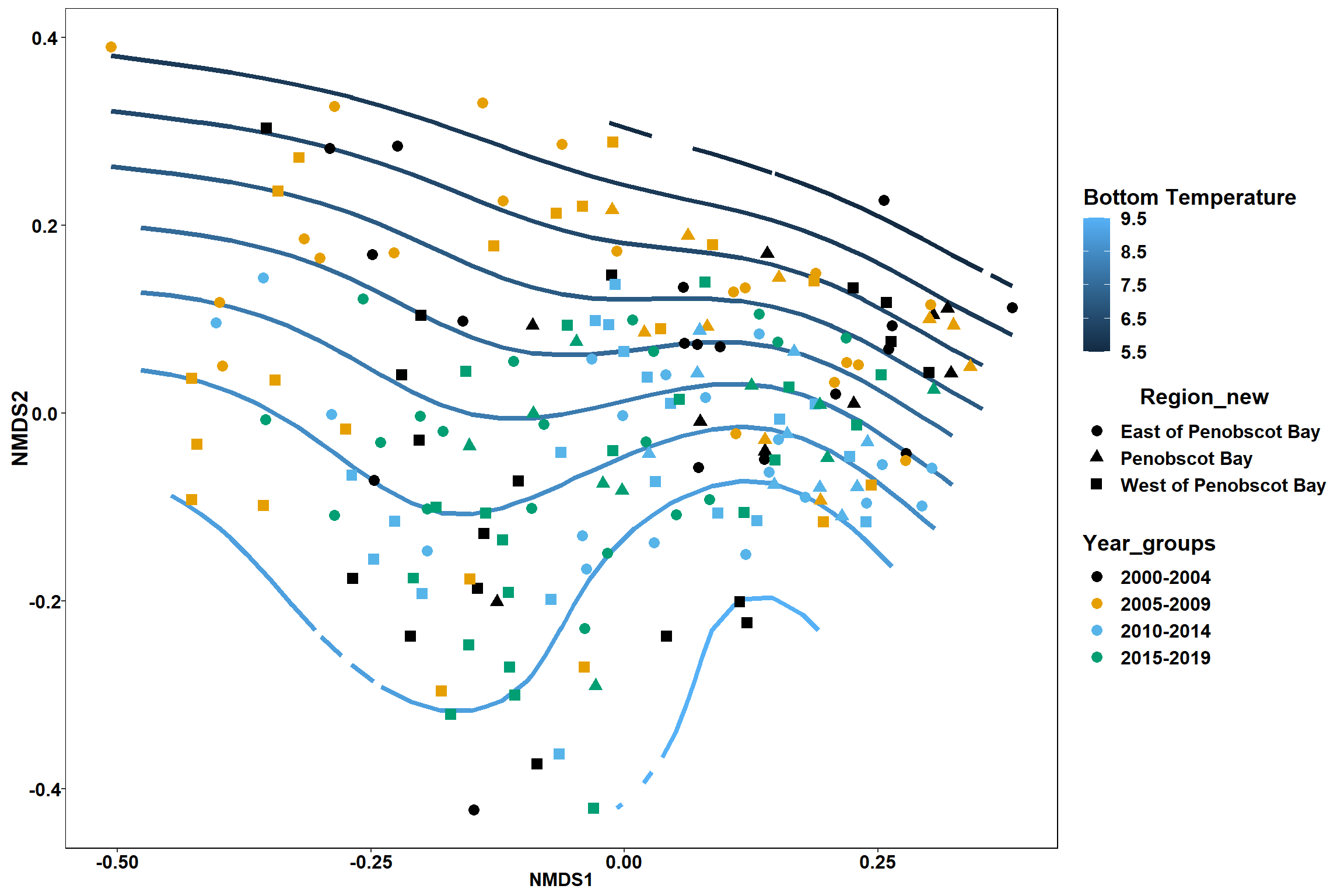
p1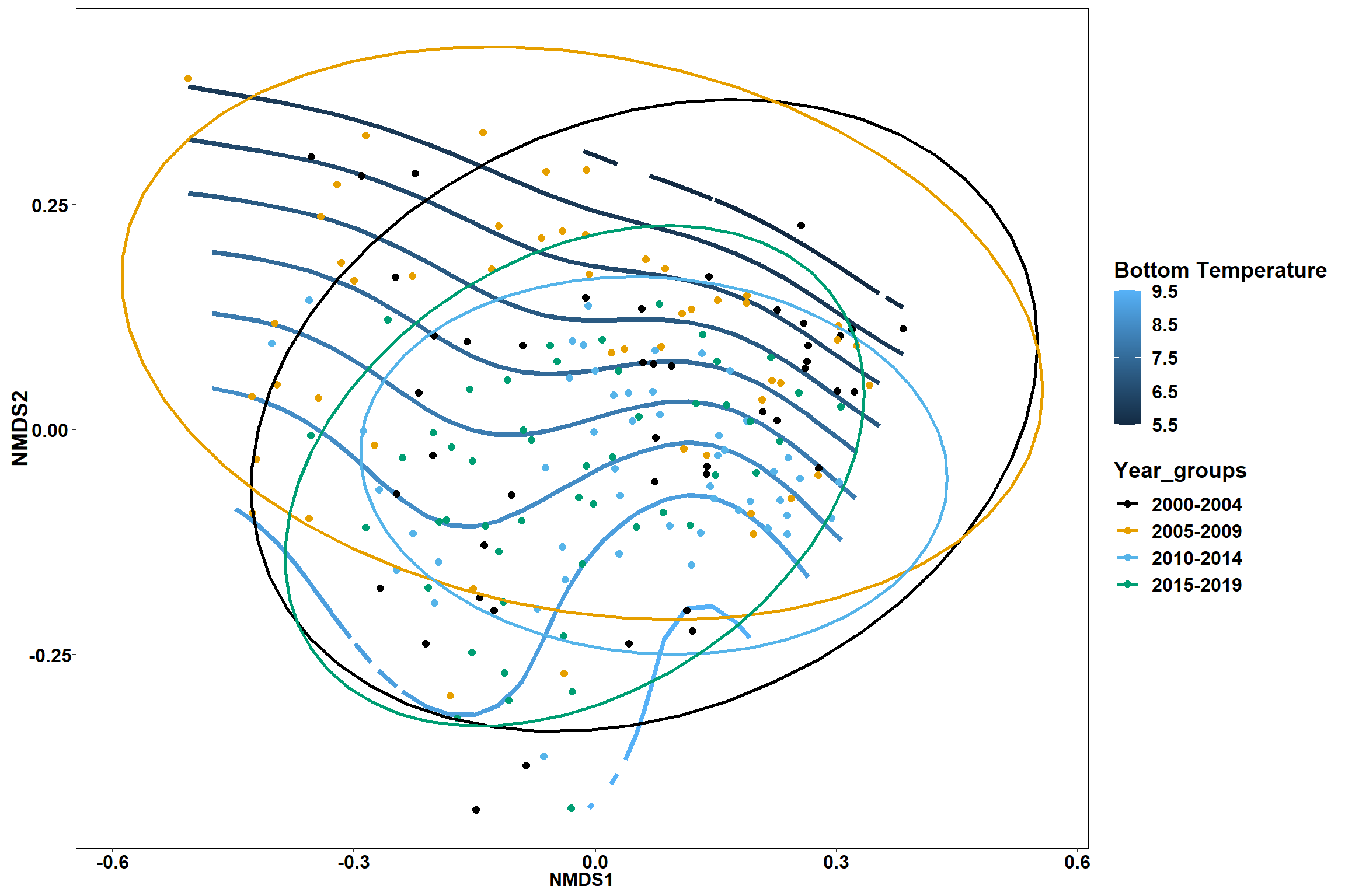
p2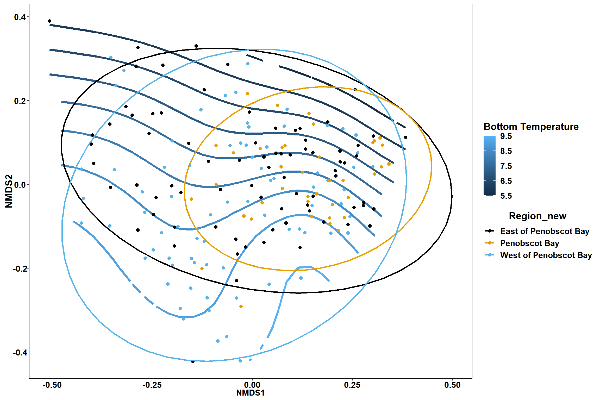
Surface temperature
surface_temp<-ordisurf(nmds, env$surface_temp)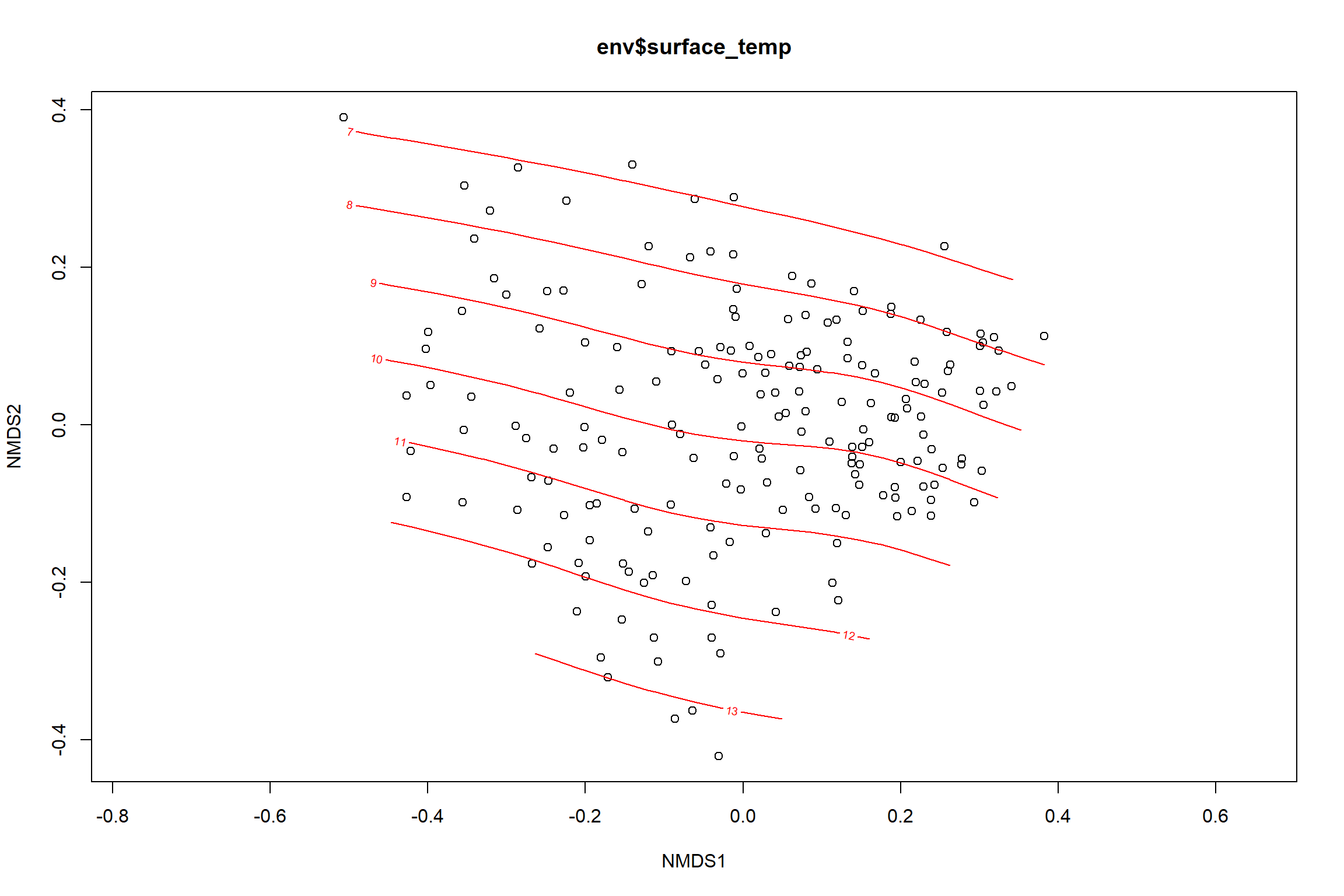
summary(surface_temp)##
## Family: gaussian
## Link function: identity
##
## Formula:
## y ~ s(x1, x2, k = 10, bs = "tp", fx = FALSE)
##
## Parametric coefficients:
## Estimate Std. Error t value Pr(>|t|)
## (Intercept) 9.7700 0.1658 58.93 <2e-16 ***
## ---
## Signif. codes: 0 '***' 0.001 '**' 0.01 '*' 0.05 '.' 0.1 ' ' 1
##
## Approximate significance of smooth terms:
## edf Ref.df F p-value
## s(x1,x2) 3.525 9 8.82 <2e-16 ***
## ---
## Signif. codes: 0 '***' 0.001 '**' 0.01 '*' 0.05 '.' 0.1 ' ' 1
##
## R-sq.(adj) = 0.296 Deviance explained = 30.9%
## -REML = 431.74 Scale est. = 5.2228 n = 190ordi.grid <- surface_temp$grid #extracts the ordisurf object
#str(ordi.grid) #it's a list though - cannot be plotted as is
ordi.mite <- expand.grid(x = ordi.grid$x, y = ordi.grid$y) #get x and ys
ordi.mite$z <- as.vector(ordi.grid$z) #unravel the matrix for the z scores
contour.vals <- data.frame(na.omit(ordi.mite)) #gets rid of the nas
p <- ggplot()+
stat_contour(data = contour.vals, aes(x, y, z=z, color = ..level..),position="identity",size=1.5)+
labs(x = "NMDS1", y = "NMDS2", color="Surface Temperature")+
new_scale_color()+
geom_point(data = data.scores, aes(NMDS1, NMDS2, color=Year_groups, shape=Region_new), size = 3 )+ scale_color_colorblind()
p1 <- ggplot()+
stat_contour(data = contour.vals, aes(x, y, z=z, color = ..level..),position="identity",size=1.5)+
labs(x = "NMDS1", y = "NMDS2", color="Surface Temperature")+
new_scale_color()+
geom_point(data = data.scores, aes(NMDS1, NMDS2, color=Year_groups), size = 2 )+stat_ellipse(data=data.scores, aes(x=NMDS1, y=NMDS2, color=Year_groups),level = 0.95,size=1)+
scale_color_colorblind()
p2 <- ggplot()+
stat_contour(data = contour.vals, aes(x, y, z=z, color = ..level..),position="identity",size=1.5)+
labs(x = "NMDS1", y = "NMDS2", color="Surface Temperature")+
new_scale_color()+
geom_point(data = data.scores, aes(NMDS1, NMDS2, color=Region_new), size = 2 )+stat_ellipse(data=data.scores, aes(x=NMDS1, y=NMDS2, color=Region_new),level = 0.95,size=1)+
scale_color_colorblind()
p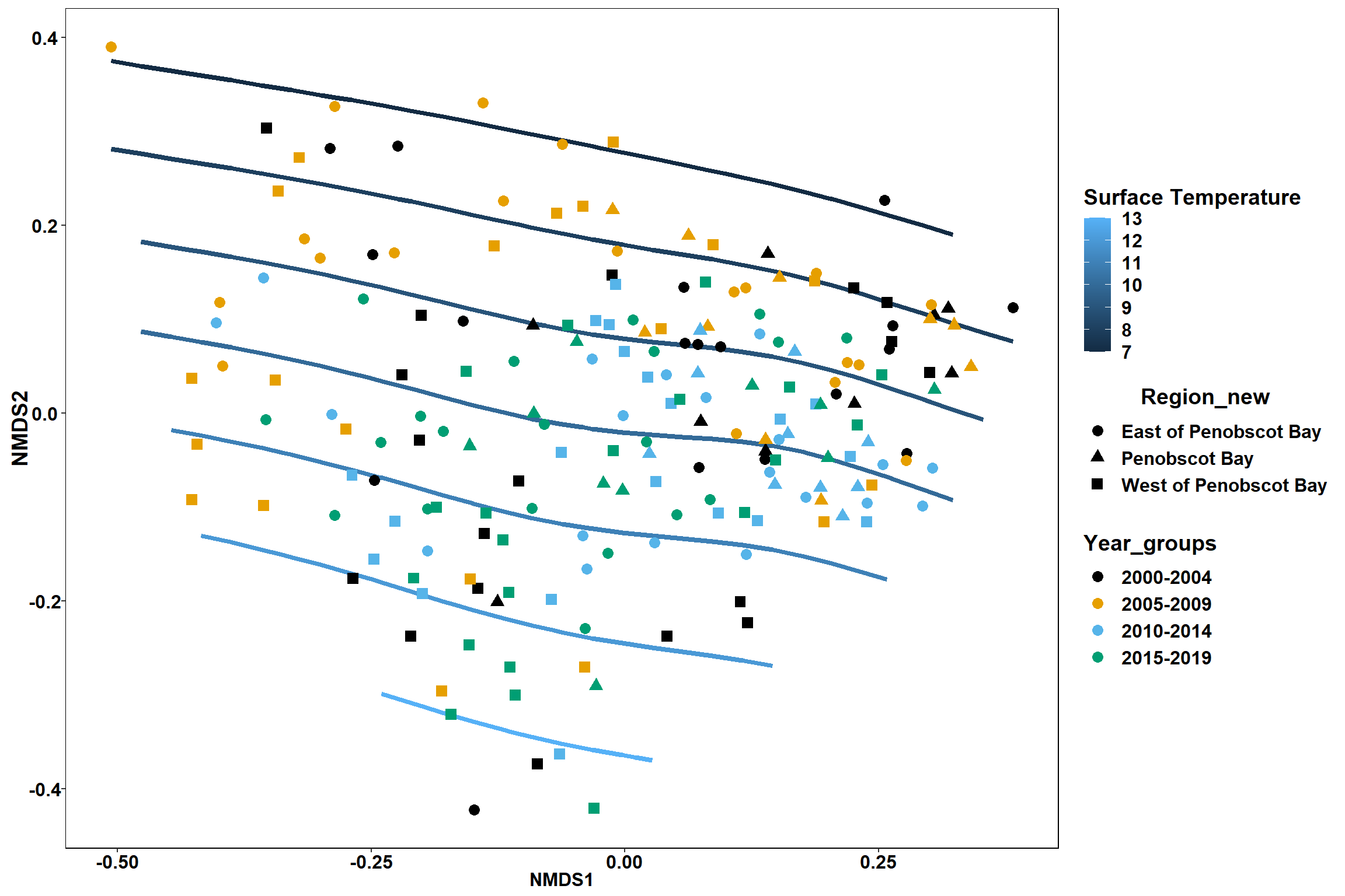
p1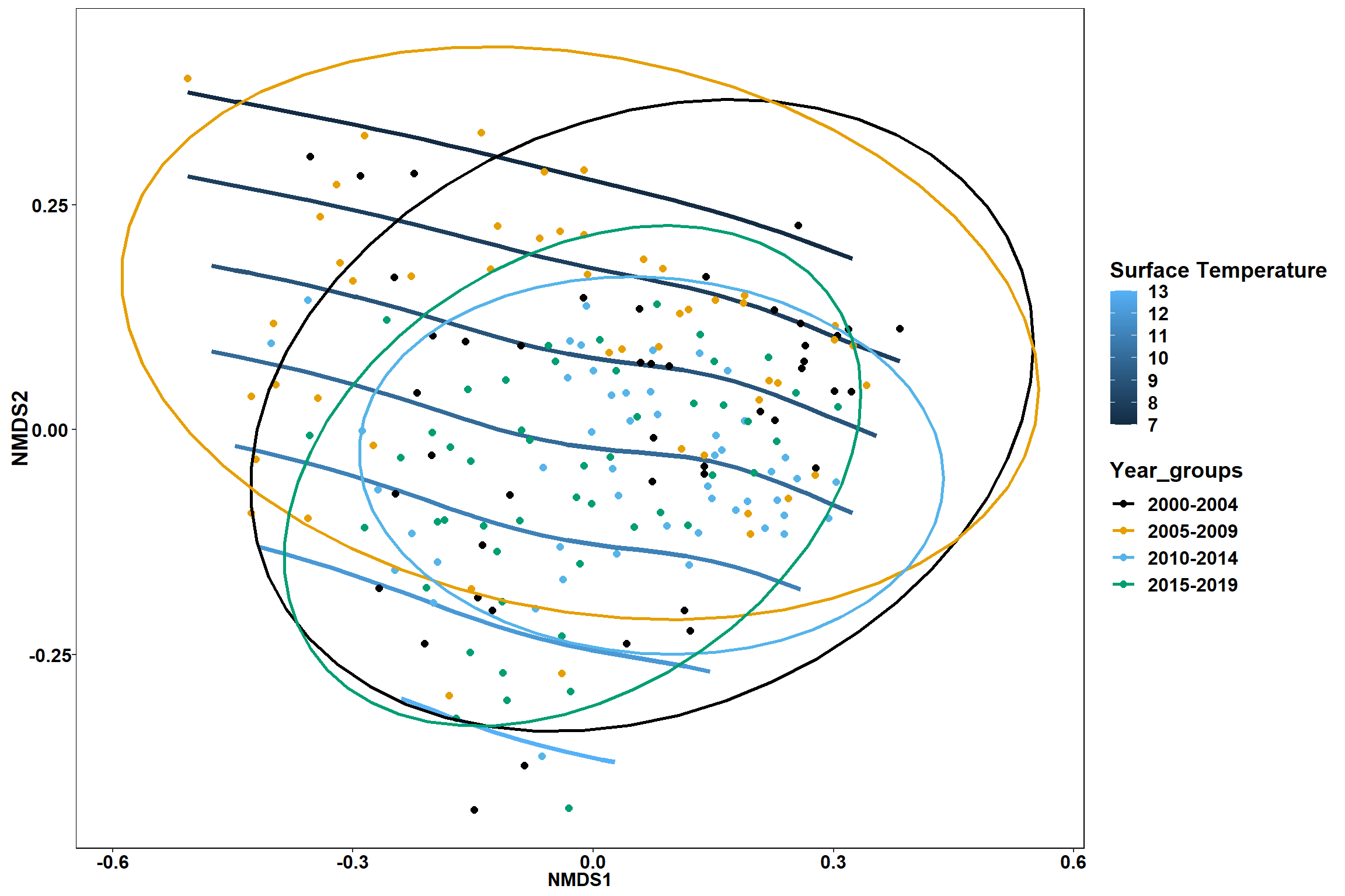
p2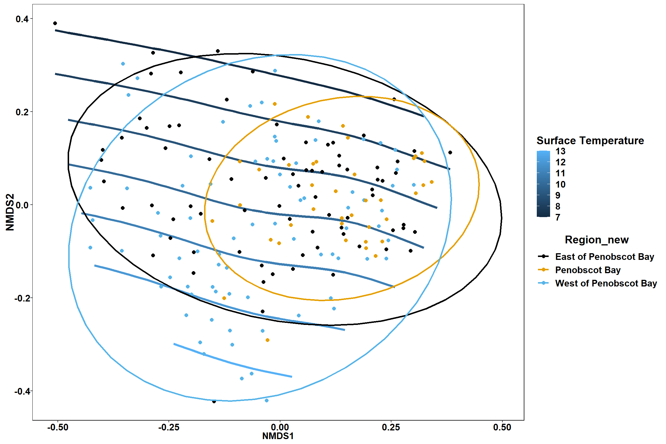
Bottom salinity
bottom_sal<-ordisurf(nmds, env$bottom_sal)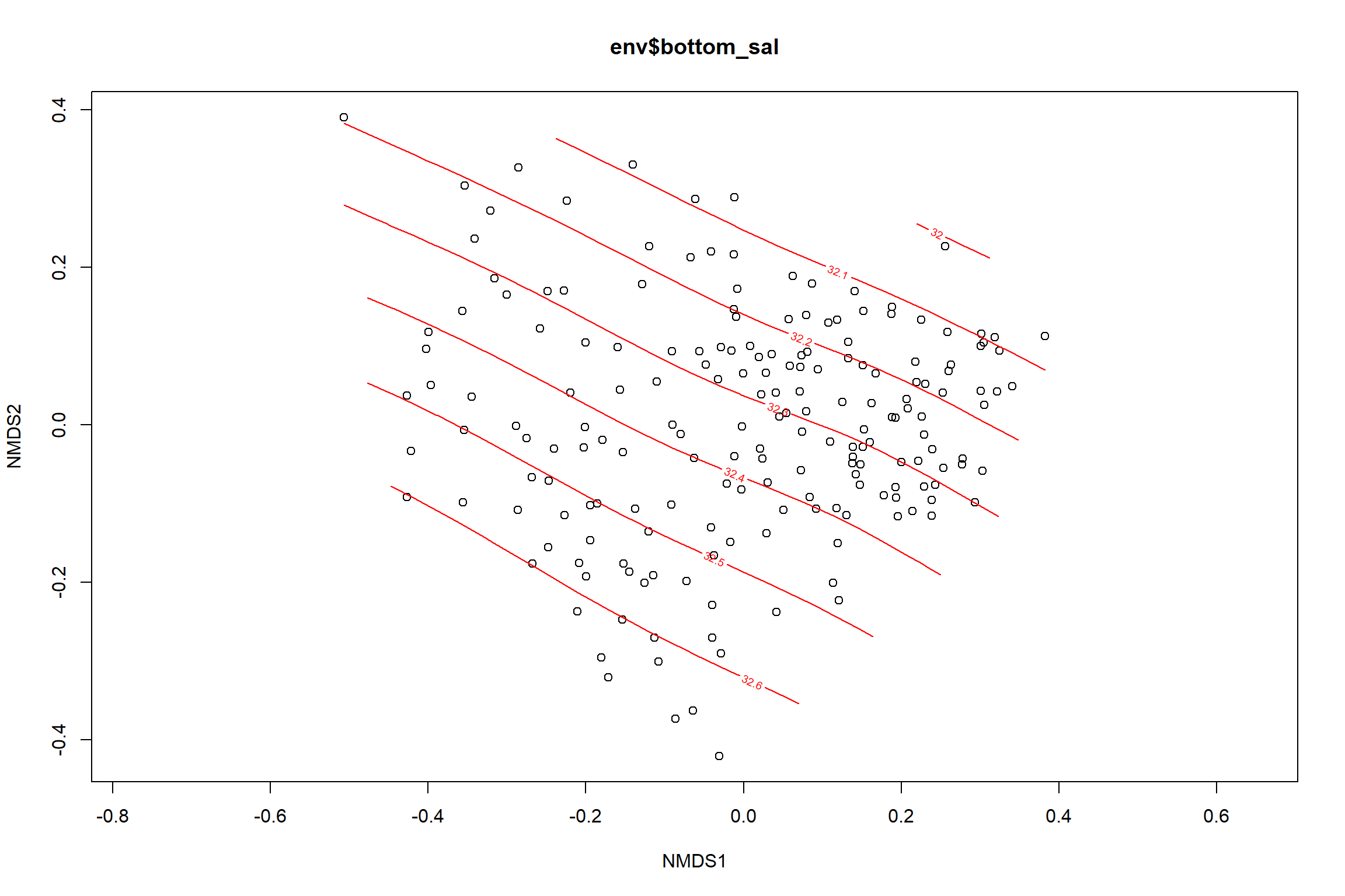
summary(bottom_sal)##
## Family: gaussian
## Link function: identity
##
## Formula:
## y ~ s(x1, x2, k = 10, bs = "tp", fx = FALSE)
##
## Parametric coefficients:
## Estimate Std. Error t value Pr(>|t|)
## (Intercept) 32.33134 0.03535 914.5 <2e-16 ***
## ---
## Signif. codes: 0 '***' 0.001 '**' 0.01 '*' 0.05 '.' 0.1 ' ' 1
##
## Approximate significance of smooth terms:
## edf Ref.df F p-value
## s(x1,x2) 2.43 9 2.341 2.76e-05 ***
## ---
## Signif. codes: 0 '***' 0.001 '**' 0.01 '*' 0.05 '.' 0.1 ' ' 1
##
## R-sq.(adj) = 0.1 Deviance explained = 11.2%
## -REML = 137.71 Scale est. = 0.23747 n = 190ordi.grid <- bottom_sal$grid #extracts the ordisurf object
#str(ordi.grid) #it's a list though - cannot be plotted as is
ordi.mite <- expand.grid(x = ordi.grid$x, y = ordi.grid$y) #get x and ys
ordi.mite$z <- as.vector(ordi.grid$z) #unravel the matrix for the z scores
contour.vals <- data.frame(na.omit(ordi.mite)) #gets rid of the nas
p <- ggplot()+
stat_contour(data = contour.vals, aes(x, y, z=z, color = ..level..),position="identity",size=1.5)+
labs(x = "NMDS1", y = "NMDS2", color="Bottom Salinity")+
new_scale_color()+
geom_point(data = data.scores, aes(NMDS1, NMDS2, color=Year_groups, shape=Region_new), size = 3 )+ scale_color_colorblind()
p1 <- ggplot()+
stat_contour(data = contour.vals, aes(x, y, z=z, color = ..level..),position="identity",size=1.5)+
labs(x = "NMDS1", y = "NMDS2", color="Bottom Salinity")+
new_scale_color()+
geom_point(data = data.scores, aes(NMDS1, NMDS2, color=Year_groups), size = 2 )+ stat_ellipse(data=data.scores, aes(x=NMDS1, y=NMDS2, color=Year_groups),level = 0.95,size=1)+
scale_color_colorblind()
p2 <- ggplot()+
stat_contour(data = contour.vals, aes(x, y, z=z, color = ..level..),position="identity",size=1.5)+
labs(x = "NMDS1", y = "NMDS2", color="Bottom Salinity")+
new_scale_color()+
geom_point(data = data.scores, aes(NMDS1, NMDS2, color=Region_new), size = 2 )+stat_ellipse(data=data.scores, aes(x=NMDS1, y=NMDS2, color=Region_new),level = 0.95,size=1)+
scale_color_colorblind()
p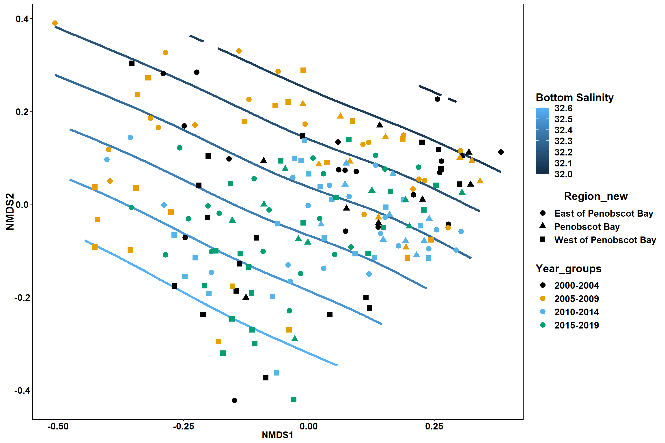
p1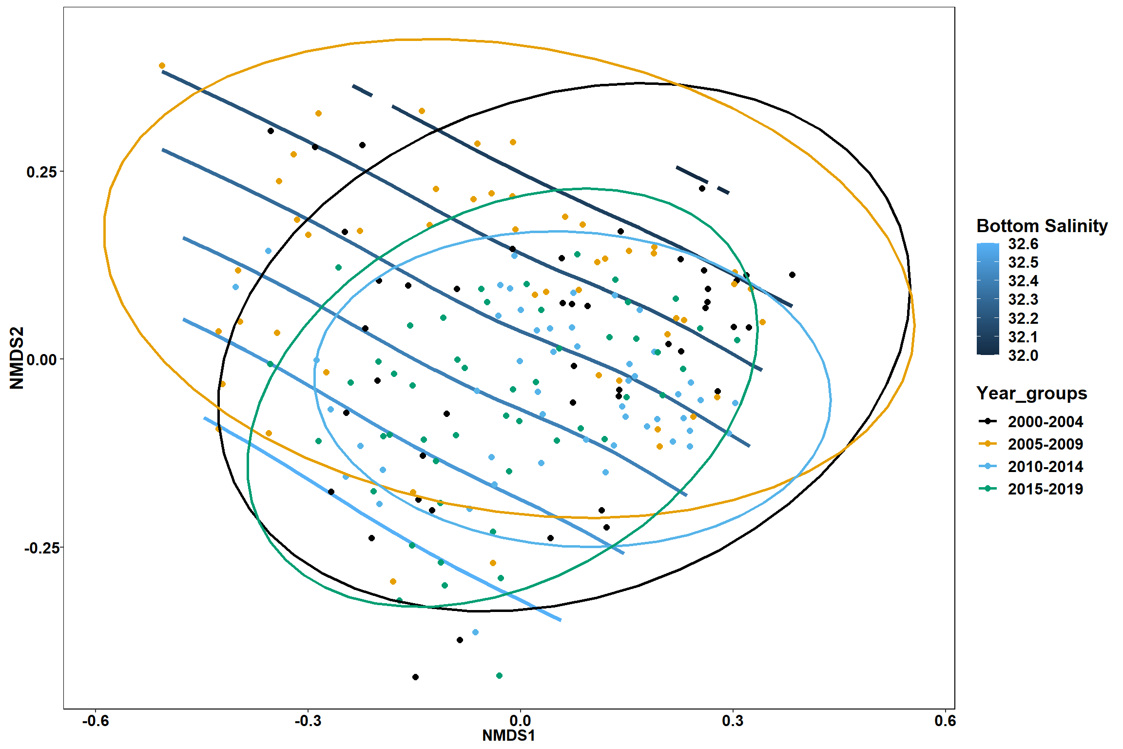
p2
Surface salinity
surface_sal<-ordisurf(nmds, env$surface_sal)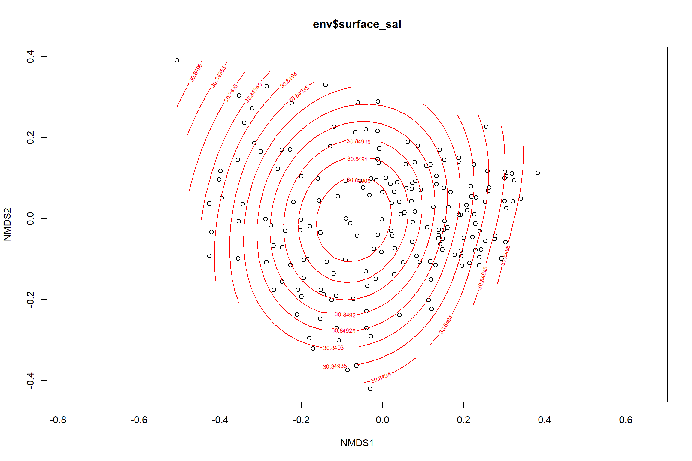
summary(surface_sal)##
## Family: gaussian
## Link function: identity
##
## Formula:
## y ~ s(x1, x2, k = 10, bs = "tp", fx = FALSE)
##
## Parametric coefficients:
## Estimate Std. Error t value Pr(>|t|)
## (Intercept) 30.8492 0.2342 131.7 <2e-16 ***
## ---
## Signif. codes: 0 '***' 0.001 '**' 0.01 '*' 0.05 '.' 0.1 ' ' 1
##
## Approximate significance of smooth terms:
## edf Ref.df F p-value
## s(x1,x2) 0.001339 9 0 0.544
##
## R-sq.(adj) = 3.94e-06 Deviance explained = 0.0011%
## -REML = 492.33 Scale est. = 10.425 n = 190ordi.grid <- surface_sal$grid #extracts the ordisurf object
#str(ordi.grid) #it's a list though - cannot be plotted as is
ordi.mite <- expand.grid(x = ordi.grid$x, y = ordi.grid$y) #get x and ys
ordi.mite$z <- as.vector(ordi.grid$z) #unravel the matrix for the z scores
contour.vals <- data.frame(na.omit(ordi.mite)) #gets rid of the nas
p <- ggplot()+
stat_contour(data = contour.vals, aes(x, y, z=z, color = ..level..),position="identity",size=1.5)+
labs(x = "NMDS1", y = "NMDS2", color="Surface Salinity")+
new_scale_color()+
geom_point(data = data.scores, aes(NMDS1, NMDS2, color=Year_groups, shape=Region_new), size = 3 )+ scale_color_colorblind()
p1 <- ggplot()+
stat_contour(data = contour.vals, aes(x, y, z=z, color = ..level..),position="identity",size=1.5)+
labs(x = "NMDS1", y = "NMDS2", color="Surface Salinity")+
new_scale_color()+
geom_point(data = data.scores, aes(NMDS1, NMDS2, color=Year_groups), size = 2 )+stat_ellipse(data=data.scores, aes(x=NMDS1, y=NMDS2, color=Year_groups),level = 0.95,size=1)+
scale_color_colorblind()
p2 <- ggplot()+
stat_contour(data = contour.vals, aes(x, y, z=z, color = ..level..),position="identity",size=1.5)+
labs(x = "NMDS1", y = "NMDS2", color="Surface Salinity")+
new_scale_color()+
geom_point(data = data.scores, aes(NMDS1, NMDS2, color=Region_new), size = 2 )+stat_ellipse(data=data.scores, aes(x=NMDS1, y=NMDS2, color=Region_new),level = 0.95,size=1)+
scale_color_colorblind()
p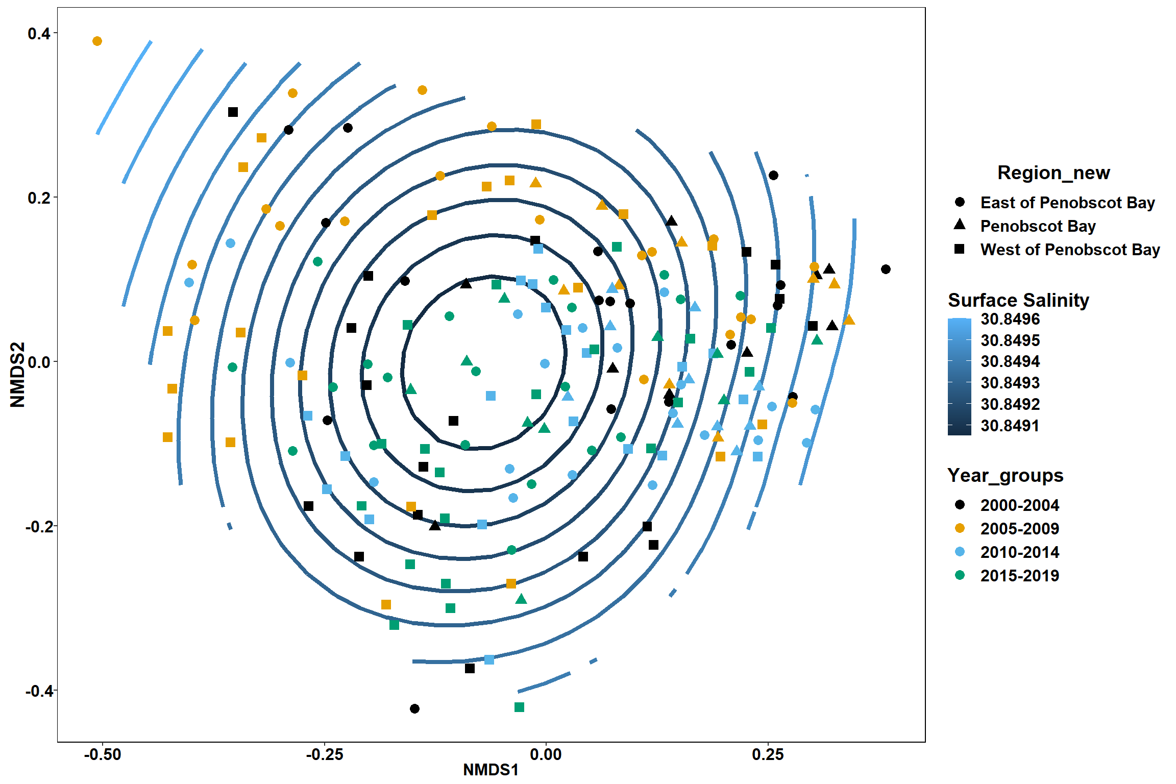
p1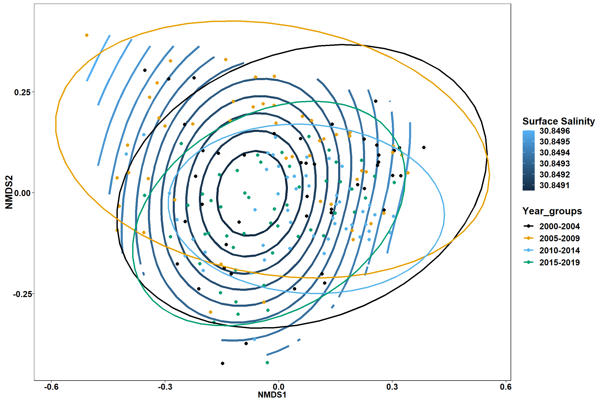
p2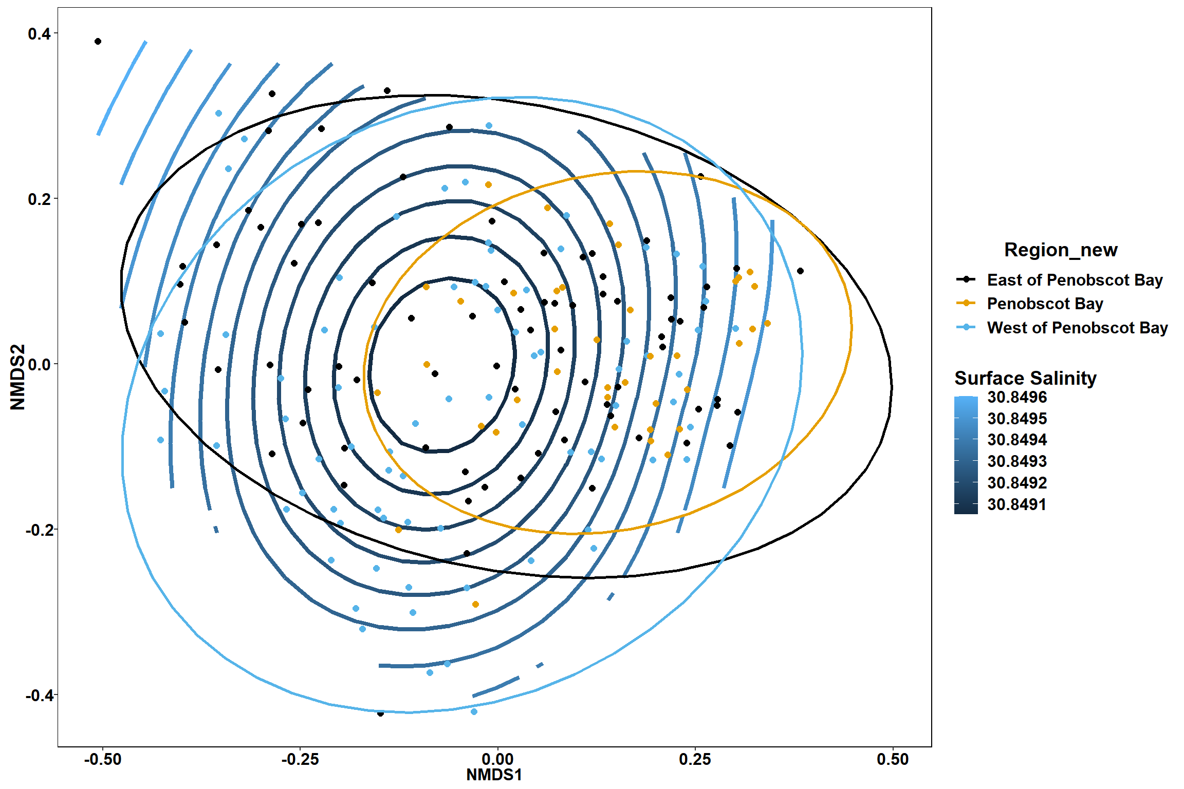
start latitude
start_lat<-ordisurf(nmds, env$start_lat)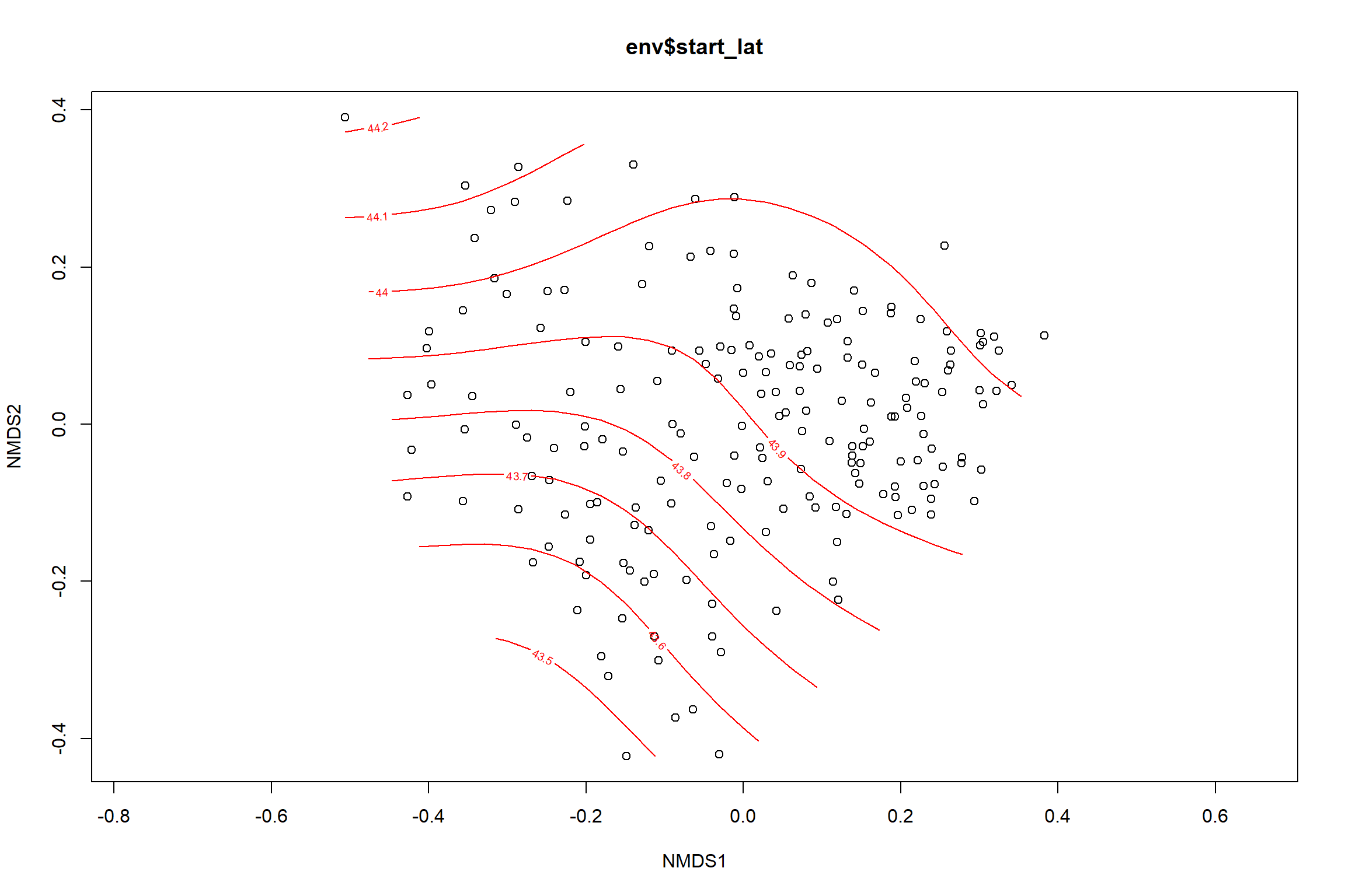
summary(start_lat)##
## Family: gaussian
## Link function: identity
##
## Formula:
## y ~ s(x1, x2, k = 10, bs = "tp", fx = FALSE)
##
## Parametric coefficients:
## Estimate Std. Error t value Pr(>|t|)
## (Intercept) 43.87499 0.02901 1512 <2e-16 ***
## ---
## Signif. codes: 0 '***' 0.001 '**' 0.01 '*' 0.05 '.' 0.1 ' ' 1
##
## Approximate significance of smooth terms:
## edf Ref.df F p-value
## s(x1,x2) 4.389 9 2.949 1.08e-05 ***
## ---
## Signif. codes: 0 '***' 0.001 '**' 0.01 '*' 0.05 '.' 0.1 ' ' 1
##
## R-sq.(adj) = 0.12 Deviance explained = 14%
## -REML = 106.86 Scale est. = 0.16413 n = 195ordi.grid <- start_lat$grid #extracts the ordisurf object
#str(ordi.grid) #it's a list though - cannot be plotted as is
ordi.mite <- expand.grid(x = ordi.grid$x, y = ordi.grid$y) #get x and ys
ordi.mite$z <- as.vector(ordi.grid$z) #unravel the matrix for the z scores
contour.vals <- data.frame(na.omit(ordi.mite)) #gets rid of the nas
p <- ggplot()+
stat_contour(data = contour.vals, aes(x, y, z=z, color = ..level..),position="identity",size=1.5)+
labs(x = "NMDS1", y = "NMDS2", color="Latitude")+
new_scale_color()+
geom_point(data = data.scores, aes(NMDS1, NMDS2, color=Year_groups, shape=Region_new), size = 3 )+ scale_color_colorblind()
p1 <- ggplot()+
stat_contour(data = contour.vals, aes(x, y, z=z, color = ..level..),position="identity",size=1.5)+
labs(x = "NMDS1", y = "NMDS2", color="Latitude")+
new_scale_color()+
geom_point(data = data.scores, aes(NMDS1, NMDS2, color=Year_groups), size = 2 )+ stat_ellipse(data=data.scores, aes(x=NMDS1, y=NMDS2, color=Year_groups),level = 0.95,size=1)+
scale_color_colorblind()
p2 <- ggplot()+
stat_contour(data = contour.vals, aes(x, y, z=z, color = ..level..),position="identity",size=1.5)+
labs(x = "NMDS1", y = "NMDS2", color="Latitude")+
new_scale_color()+
geom_point(data = data.scores, aes(NMDS1, NMDS2, color=Region_new), size = 2 )+ stat_ellipse(data=data.scores, aes(x=NMDS1, y=NMDS2, color=Region_new),level = 0.95,size=1)+
scale_color_colorblind()
p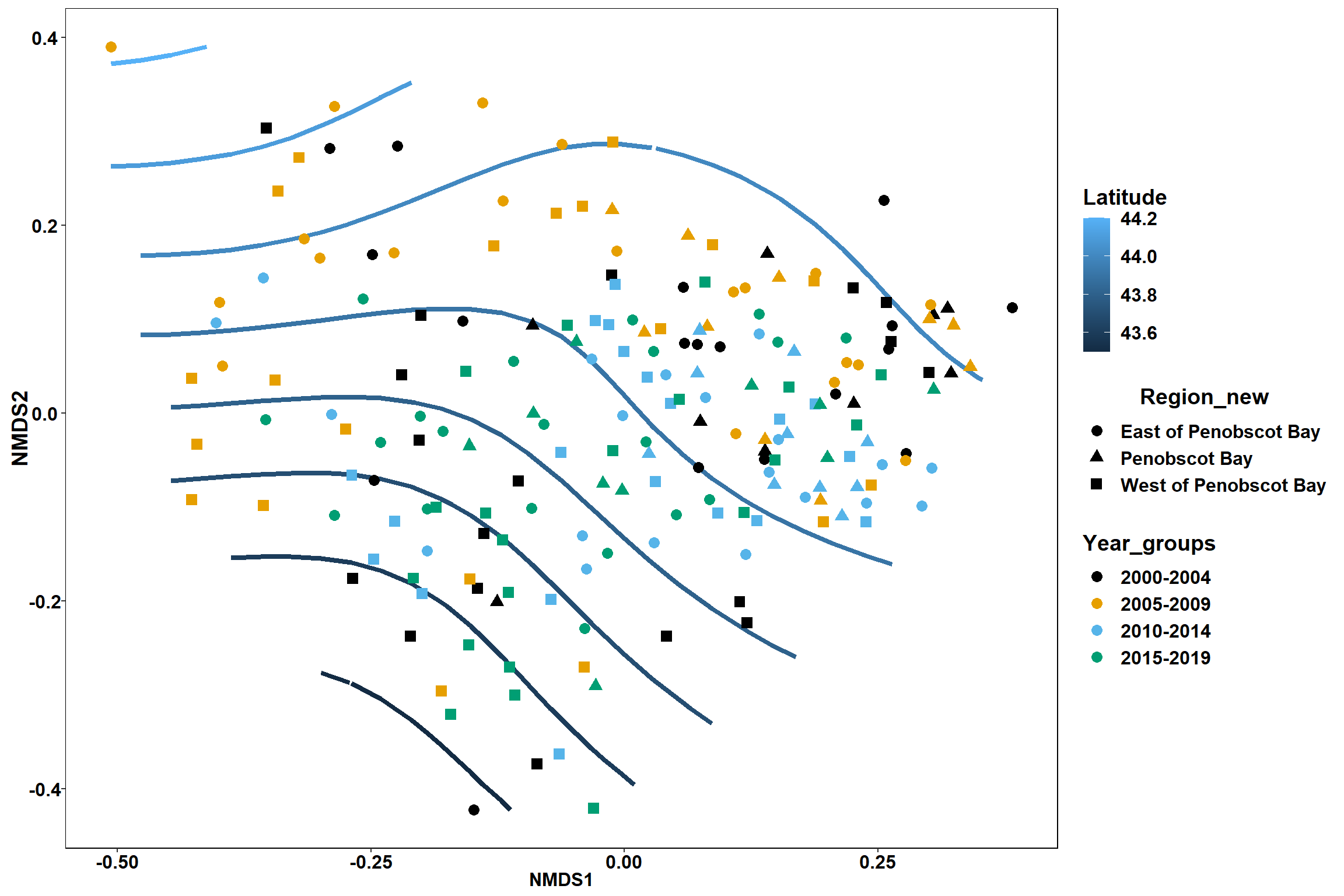
p1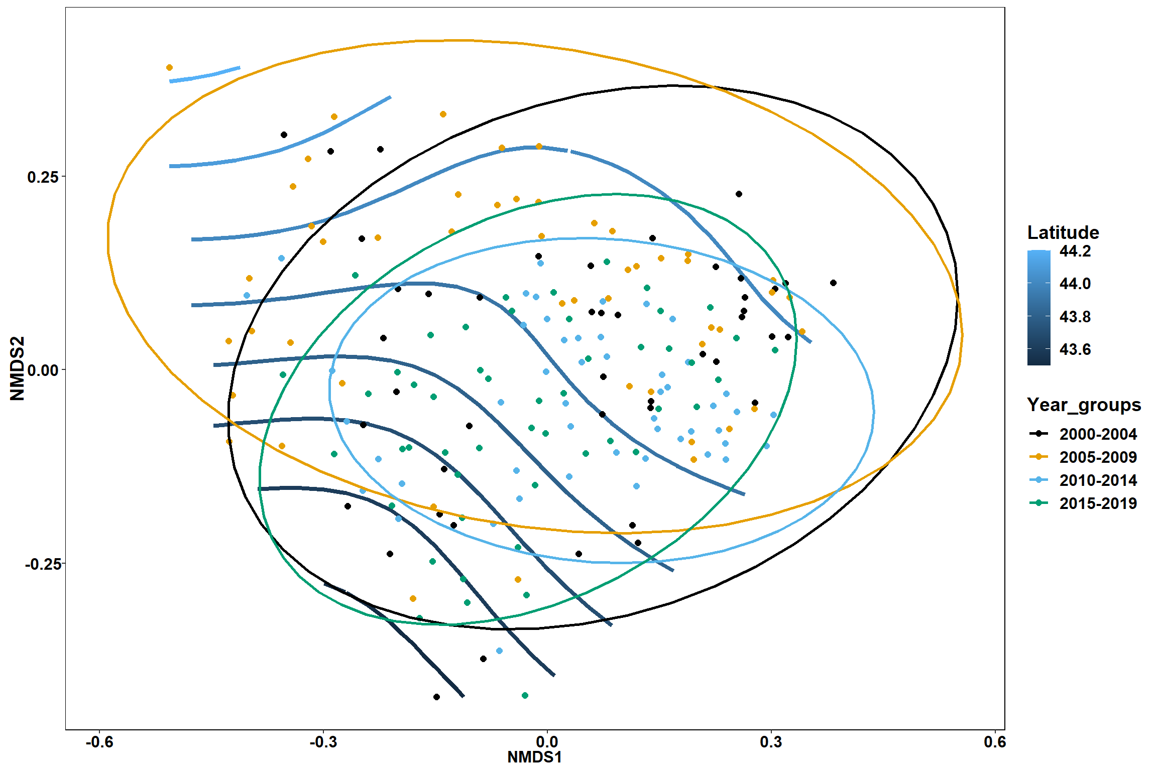
p2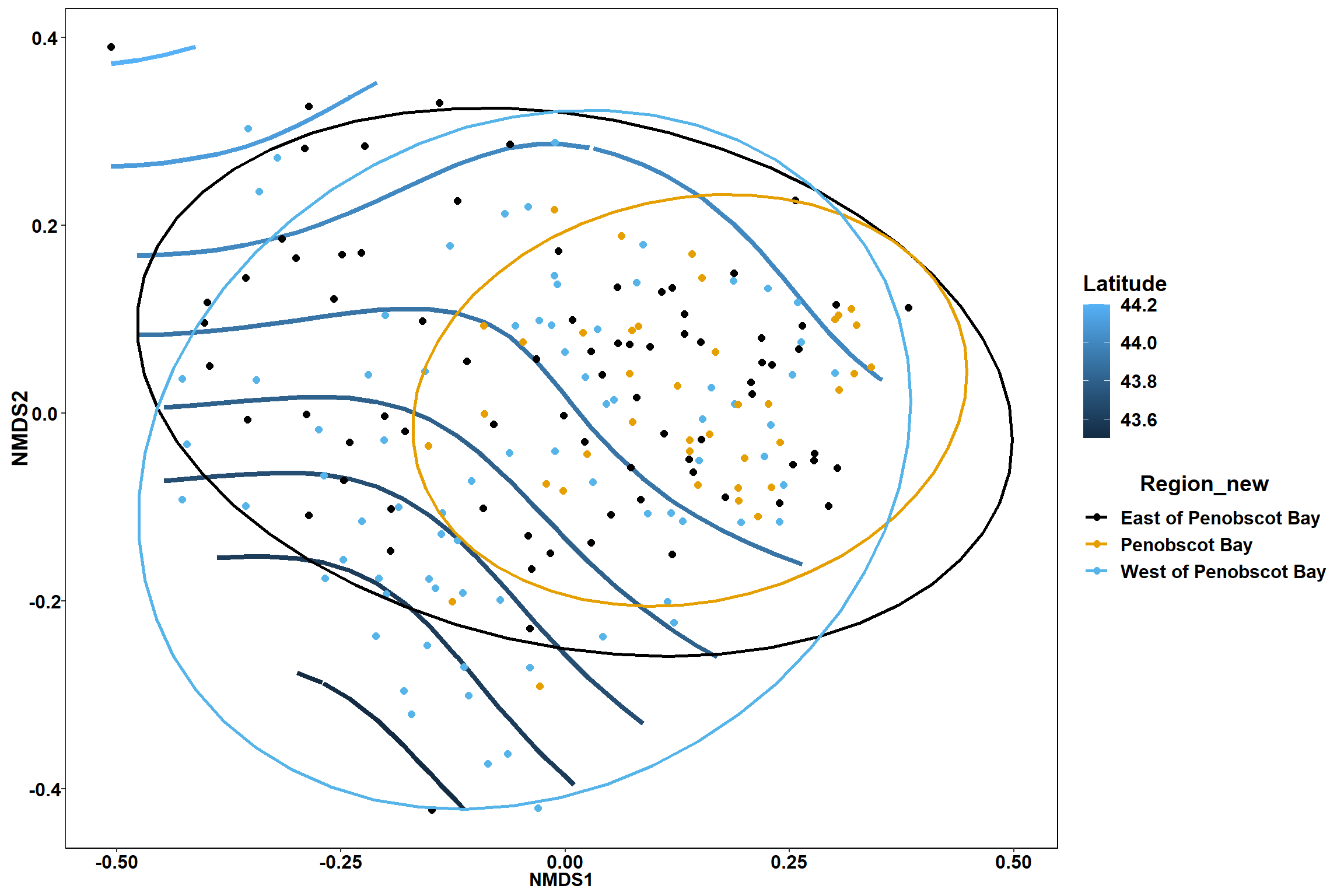
start longitude
start_long<-ordisurf(nmds, env$start_long)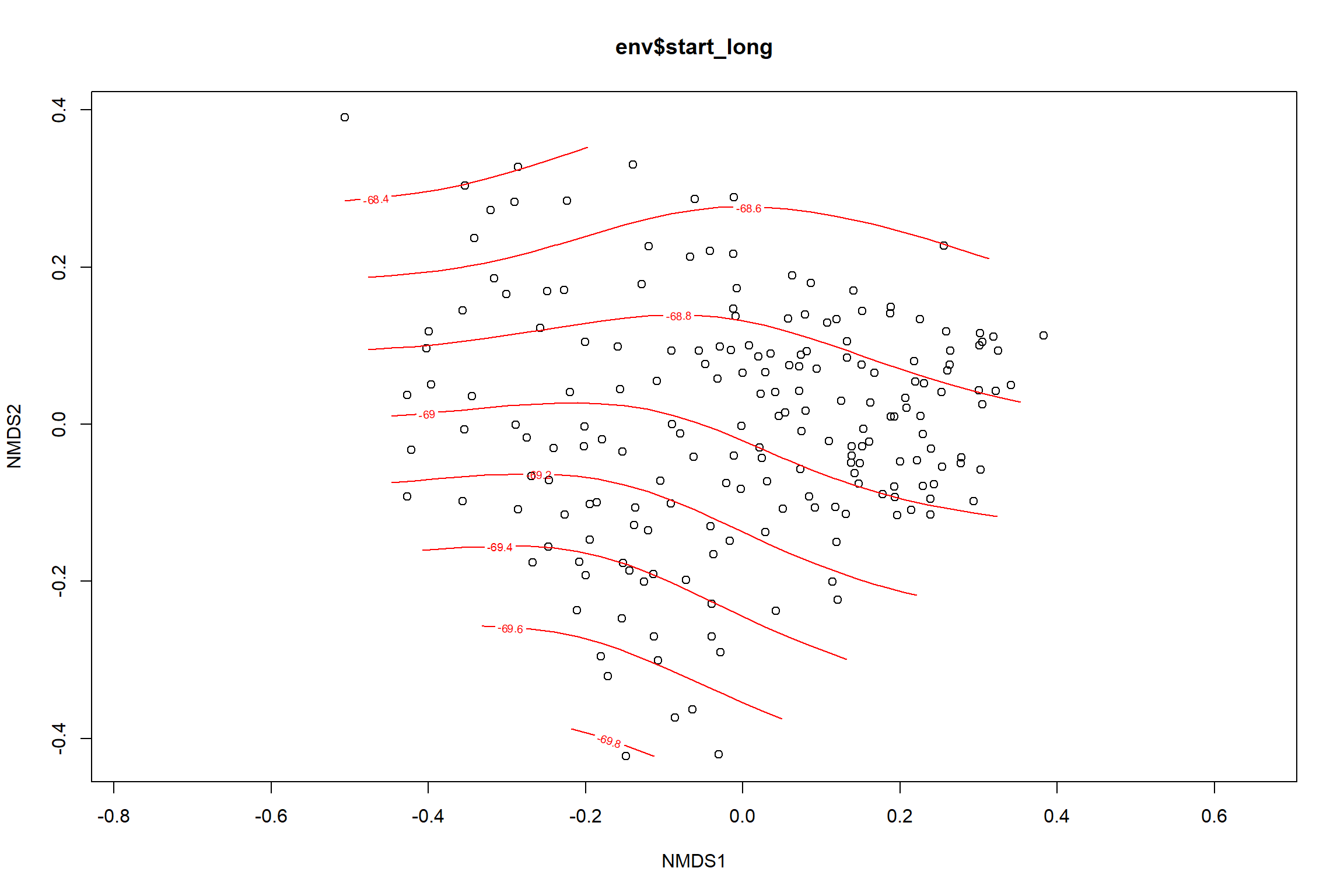
summary(start_long)##
## Family: gaussian
## Link function: identity
##
## Formula:
## y ~ s(x1, x2, k = 10, bs = "tp", fx = FALSE)
##
## Parametric coefficients:
## Estimate Std. Error t value Pr(>|t|)
## (Intercept) -68.97337 0.07037 -980.2 <2e-16 ***
## ---
## Signif. codes: 0 '***' 0.001 '**' 0.01 '*' 0.05 '.' 0.1 ' ' 1
##
## Approximate significance of smooth terms:
## edf Ref.df F p-value
## s(x1,x2) 3.26 9 2.083 0.000136 ***
## ---
## Signif. codes: 0 '***' 0.001 '**' 0.01 '*' 0.05 '.' 0.1 ' ' 1
##
## R-sq.(adj) = 0.0881 Deviance explained = 10.3%
## -REML = 277.67 Scale est. = 0.96557 n = 195ordi.grid <- start_long$grid #extracts the ordisurf object
#str(ordi.grid) #it's a list though - cannot be plotted as is
ordi.mite <- expand.grid(x = ordi.grid$x, y = ordi.grid$y) #get x and ys
ordi.mite$z <- as.vector(ordi.grid$z) #unravel the matrix for the z scores
contour.vals <- data.frame(na.omit(ordi.mite)) #gets rid of the nas
p <- ggplot()+
stat_contour(data = contour.vals, aes(x, y, z=z, color = ..level..),position="identity",size=1.5)+
labs(x = "NMDS1", y = "NMDS2", color="Longitude")+
new_scale_color()+
geom_point(data = data.scores, aes(NMDS1, NMDS2, color=Year_groups, shape=Region_new), size = 3 )+ scale_color_colorblind()
p1 <- ggplot()+
stat_contour(data = contour.vals, aes(x, y, z=z, color = ..level..),position="identity",size=1.5)+
labs(x = "NMDS1", y = "NMDS2", color="Longitude")+
new_scale_color()+
geom_point(data = data.scores, aes(NMDS1, NMDS2, color=Year_groups), size = 2 )+stat_ellipse(data=data.scores, aes(x=NMDS1, y=NMDS2, color=Year_groups),level = 0.95,size=1)+
scale_color_colorblind()
p2 <- ggplot()+
stat_contour(data = contour.vals, aes(x, y, z=z, color = ..level..),position="identity",size=1.5)+
labs(x = "NMDS1", y = "NMDS2", color="Longitude")+
new_scale_color()+
geom_point(data = data.scores, aes(NMDS1, NMDS2, color=Region_new), size = 2 )+stat_ellipse(data=data.scores, aes(x=NMDS1, y=NMDS2, color=Region_new),level = 0.95,size=1)+
scale_color_colorblind()
p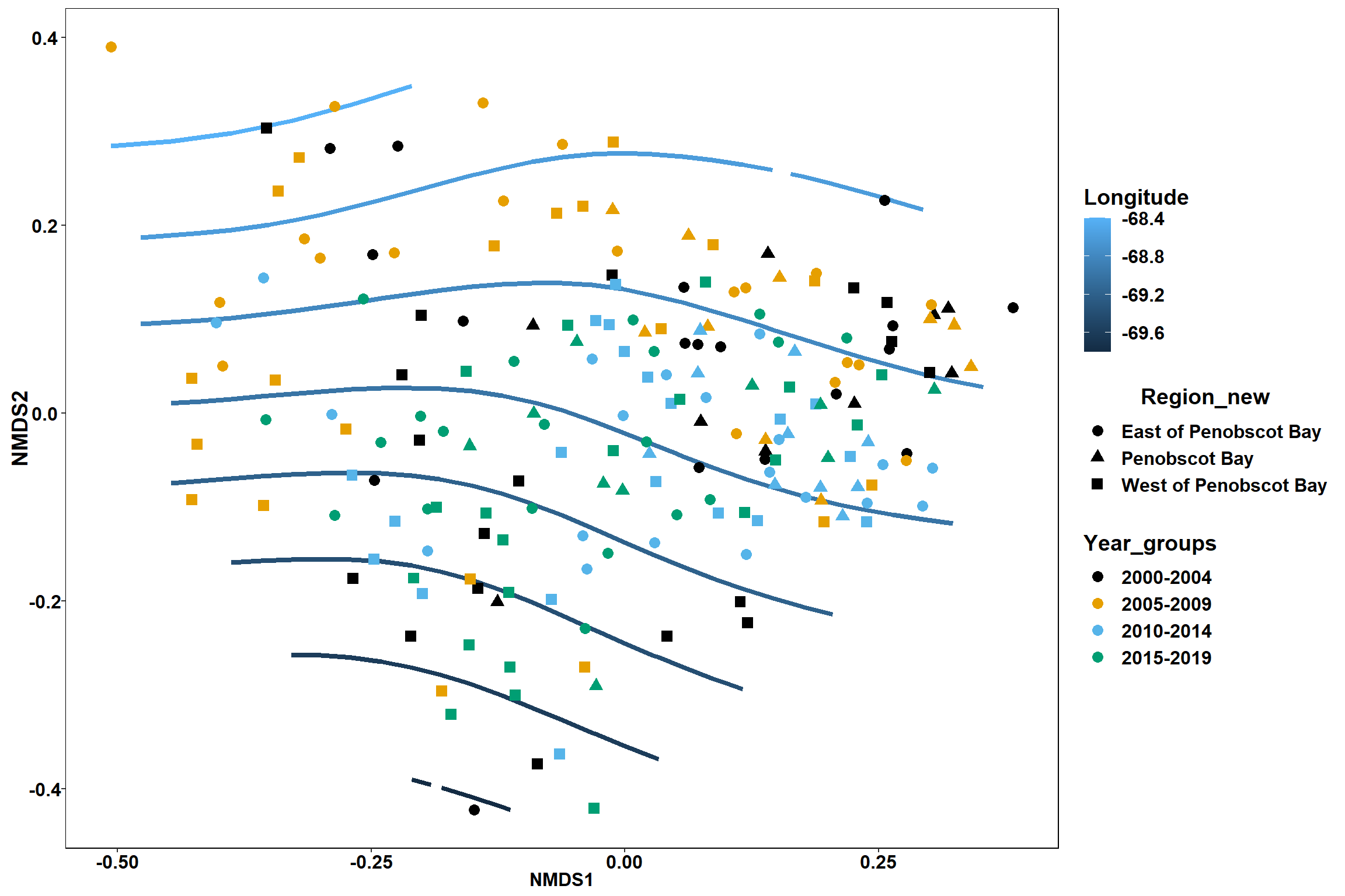
p1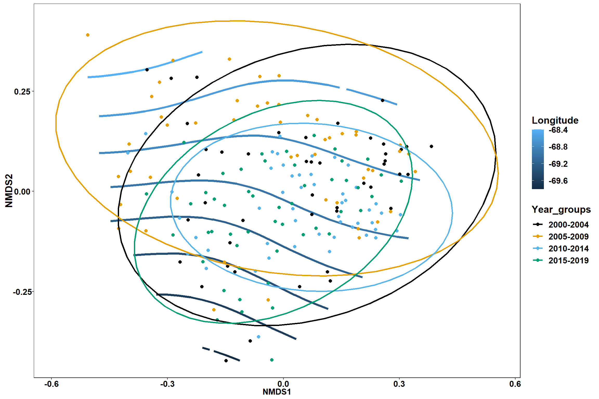
p2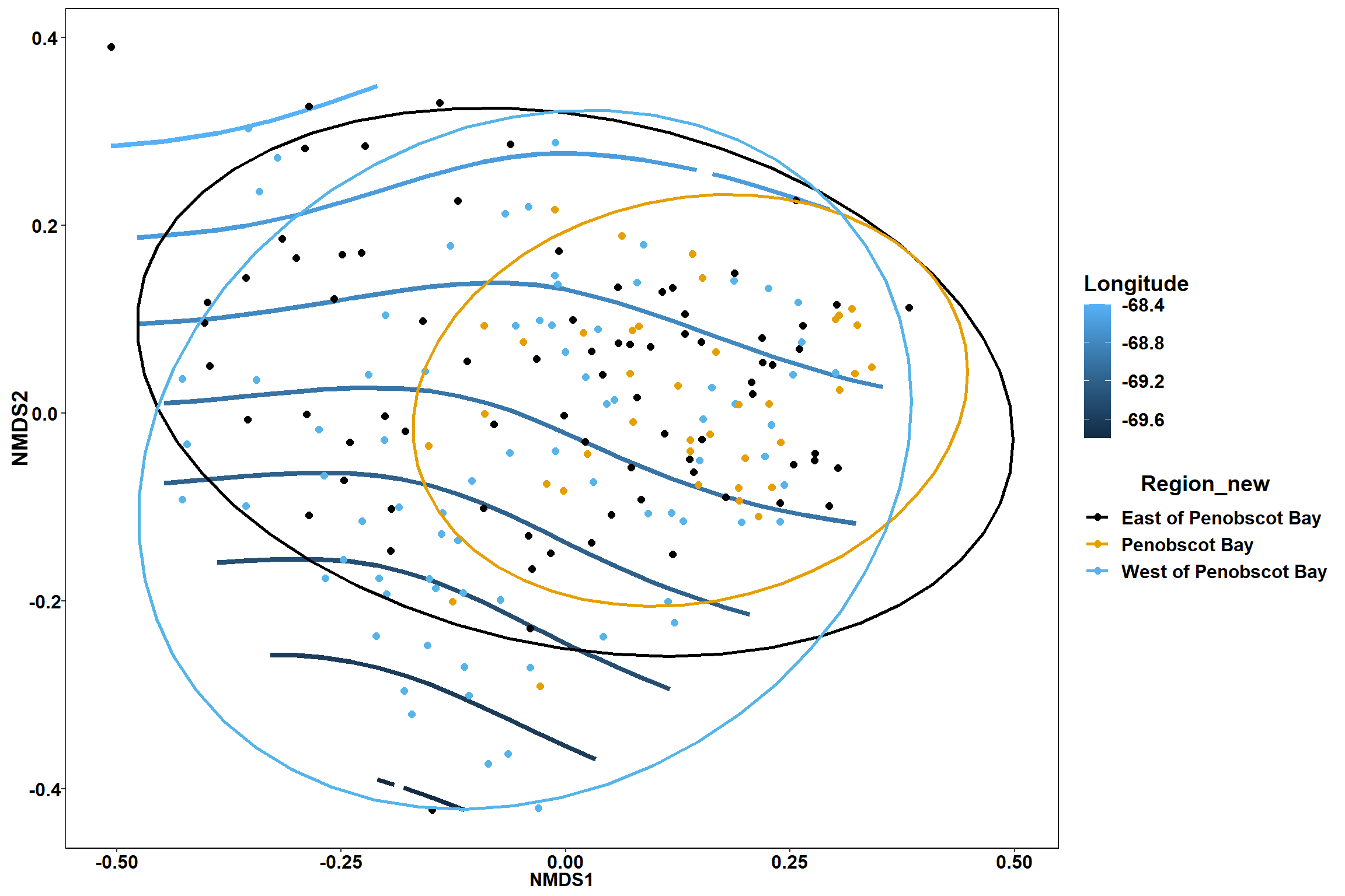
start depth
start_depth<-ordisurf(nmds, env$start_depth)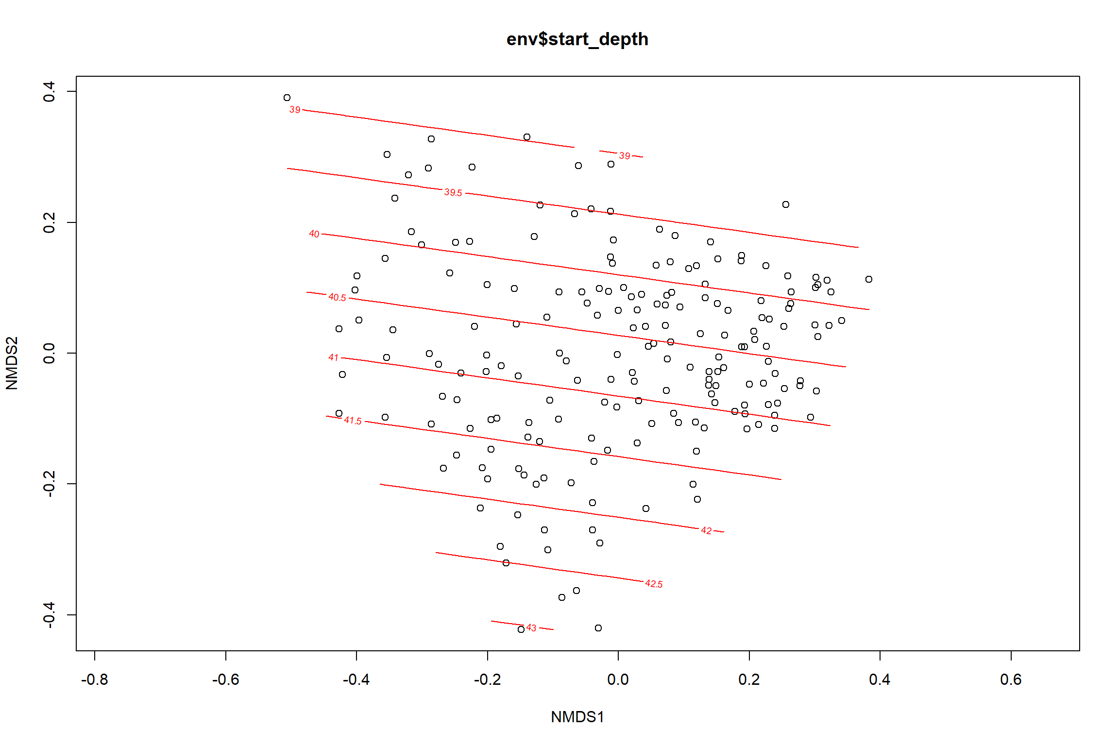
summary(start_depth)##
## Family: gaussian
## Link function: identity
##
## Formula:
## y ~ s(x1, x2, k = 10, bs = "tp", fx = FALSE)
##
## Parametric coefficients:
## Estimate Std. Error t value Pr(>|t|)
## (Intercept) 40.6472 0.3159 128.7 <2e-16 ***
## ---
## Signif. codes: 0 '***' 0.001 '**' 0.01 '*' 0.05 '.' 0.1 ' ' 1
##
## Approximate significance of smooth terms:
## edf Ref.df F p-value
## s(x1,x2) 1.608 9 0.907 0.00708 **
## ---
## Signif. codes: 0 '***' 0.001 '**' 0.01 '*' 0.05 '.' 0.1 ' ' 1
##
## R-sq.(adj) = 0.0404 Deviance explained = 4.83%
## -REML = 567.47 Scale est. = 19.46 n = 195ordi.grid <- start_depth$grid #extracts the ordisurf object
#str(ordi.grid) #it's a list though - cannot be plotted as is
ordi.mite <- expand.grid(x = ordi.grid$x, y = ordi.grid$y) #get x and ys
ordi.mite$z <- as.vector(ordi.grid$z) #unravel the matrix for the z scores
contour.vals <- data.frame(na.omit(ordi.mite)) #gets rid of the nas
p <- ggplot()+
stat_contour(data = contour.vals, aes(x, y, z=z, color = ..level..),position="identity",size=1.5)+
labs(x = "NMDS1", y = "NMDS2", color="Depth")+
new_scale_color()+
geom_point(data = data.scores, aes(NMDS1, NMDS2, color=Year_groups, shape=Region_new), size = 3 )+ scale_color_colorblind()
p1 <- ggplot()+
stat_contour(data = contour.vals, aes(x, y, z=z, color = ..level..),position="identity",size=1.5)+
labs(x = "NMDS1", y = "NMDS2", color="Depth")+
new_scale_color()+
geom_point(data = data.scores, aes(NMDS1, NMDS2, color=Year_groups), size = 2 )+stat_ellipse(data=data.scores, aes(x=NMDS1, y=NMDS2, color=Year_groups),level = 0.95,size=1)+
scale_color_colorblind()
p2 <- ggplot()+
stat_contour(data = contour.vals, aes(x, y, z=z, color = ..level..),position="identity",size=1.5)+
labs(x = "NMDS1", y = "NMDS2", color="Depth")+
new_scale_color()+
geom_point(data = data.scores, aes(NMDS1, NMDS2, color=Region_new), size = 2 )+stat_ellipse(data=data.scores, aes(x=NMDS1, y=NMDS2, color=Region_new),level = 0.95,size=1)+
scale_color_colorblind()
p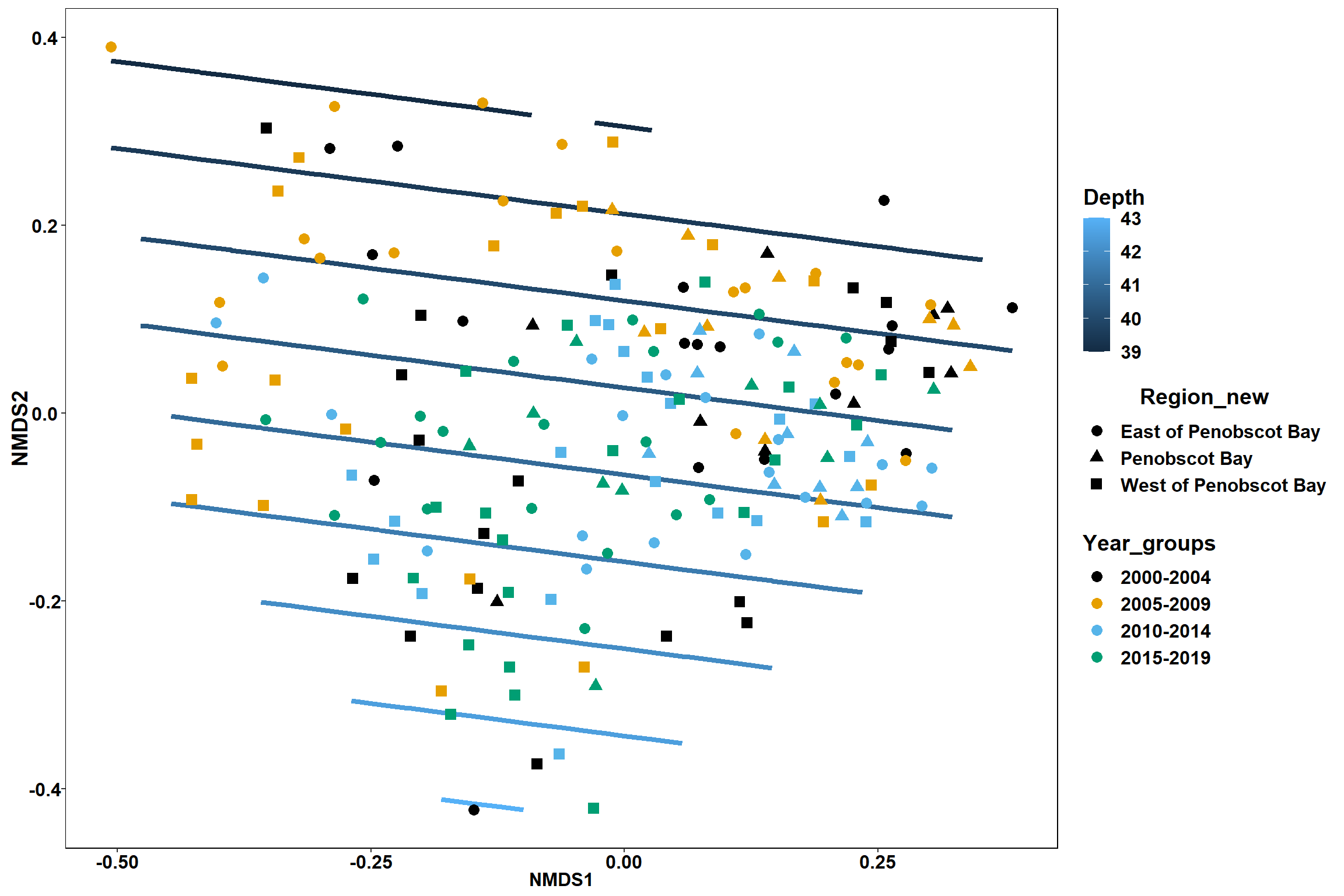
p1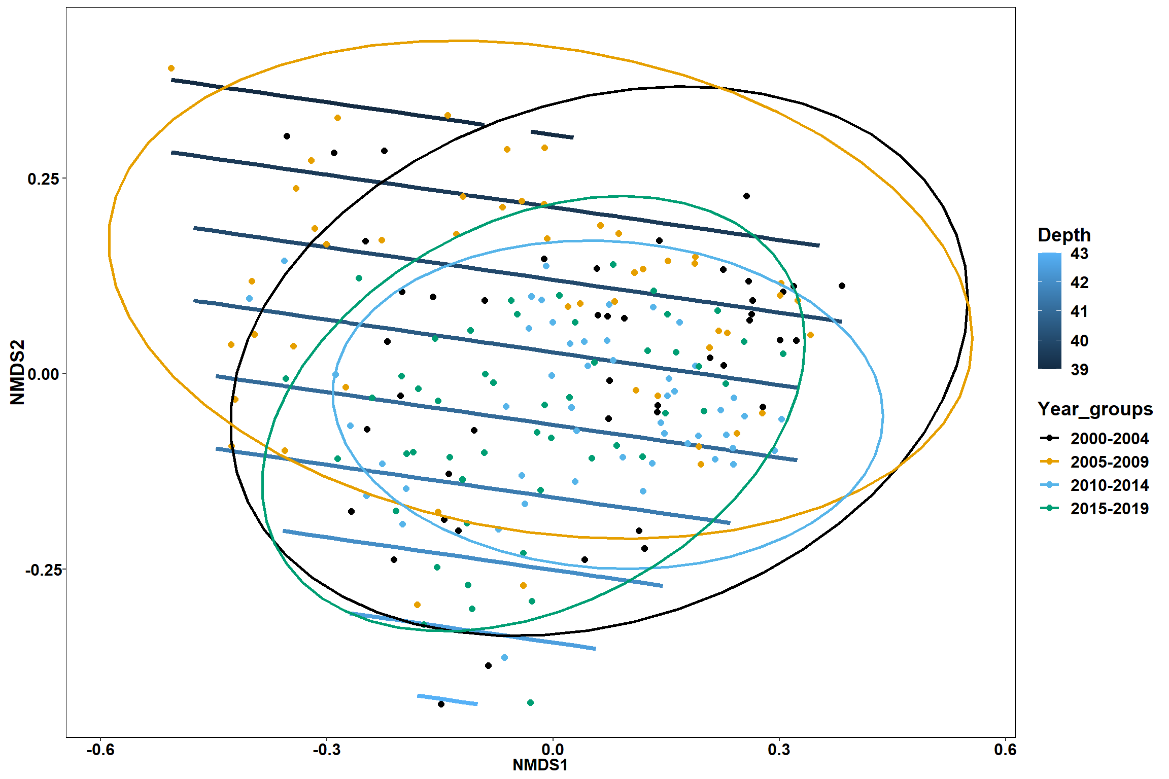
p2