Shannon-Weiner diversity
County specified data
shannon<-group_by(landings_total, year,county)%>%
mutate(total=sum(weight), prop=weight/total)%>%
summarise(shannon=-1*(sum(prop*log(prop))))
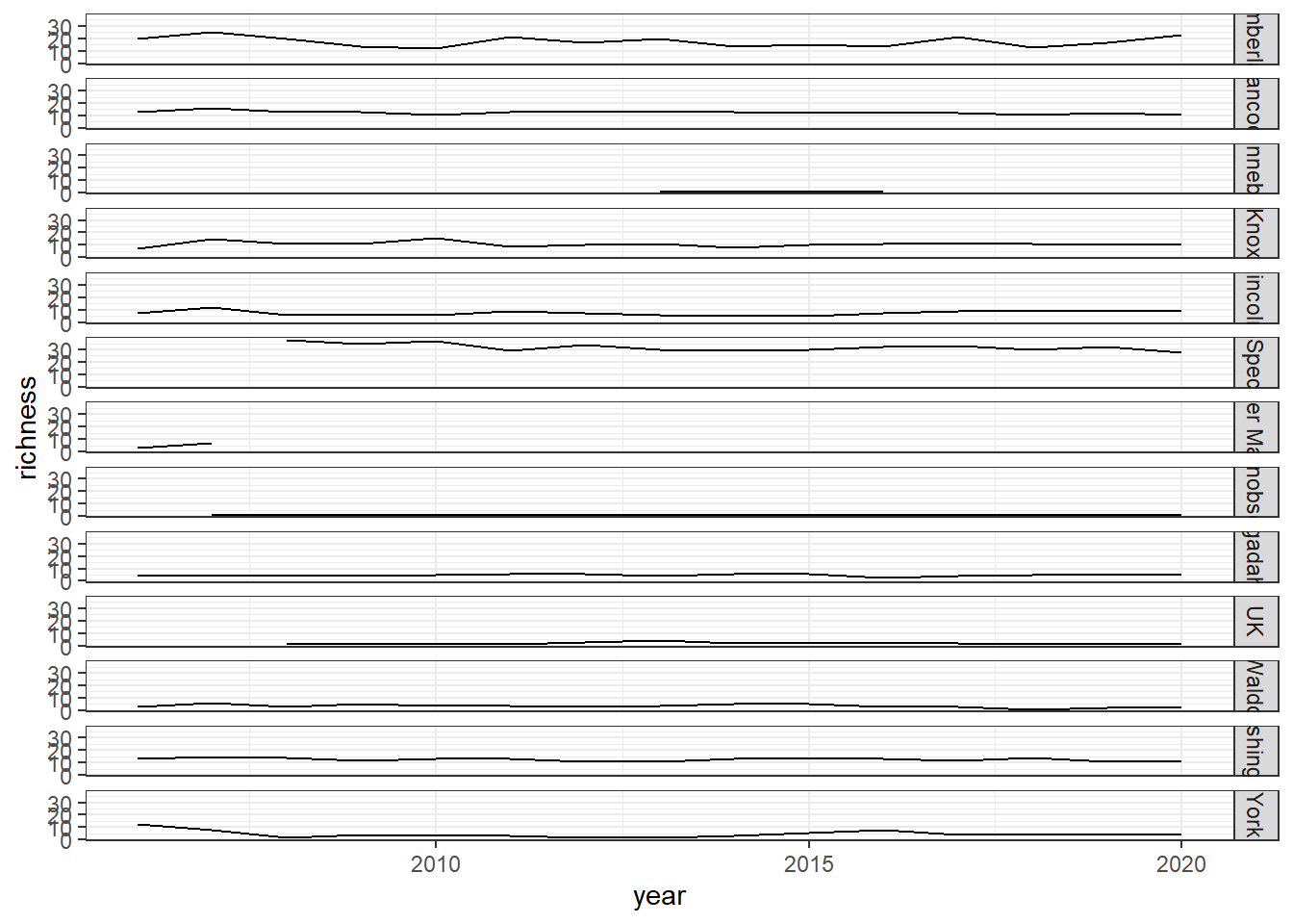
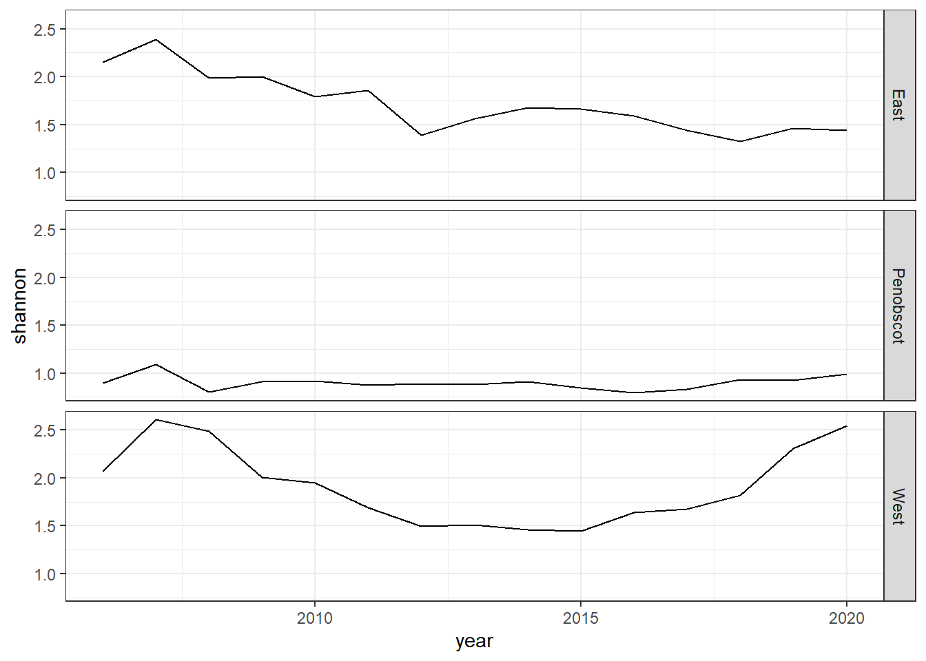
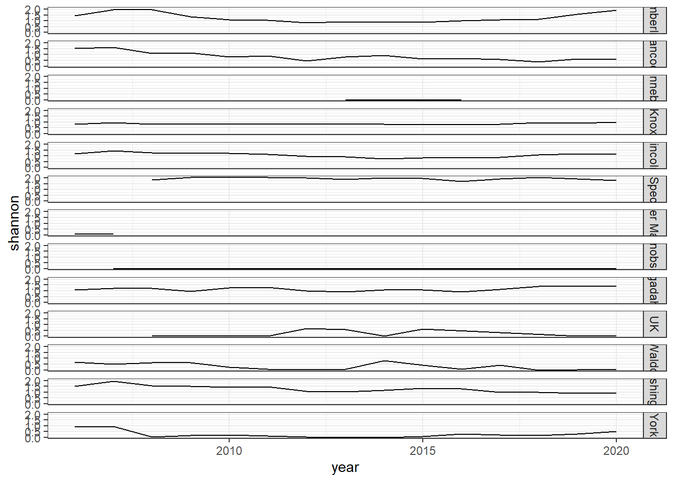
ggplot()+geom_line(data=shannon, aes(year, shannon))+
facet_grid(rows=vars(county))+theme_bw()
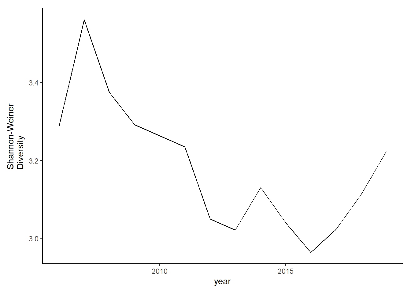
shannon<-group_by(landings_total, year,species)%>%
mutate(species_total=sum(weight))%>%
group_by(year)%>%
mutate(total=sum(species_total),prop=species_total/total)%>%
summarise(shannon=-1*(sum(prop*log(prop))))
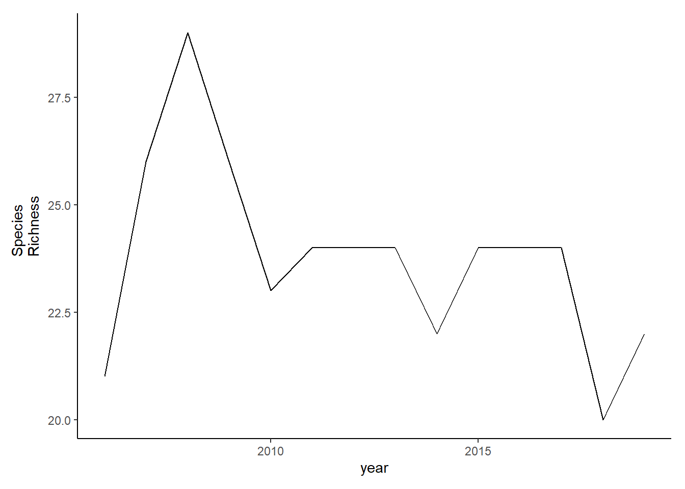
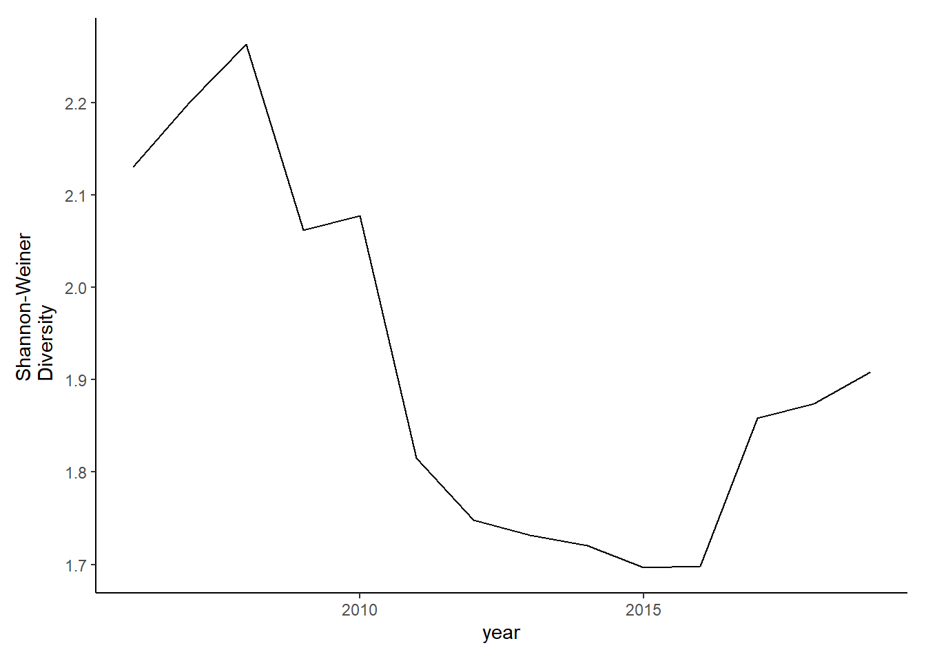
diversity<-ggplot()+geom_line(data=subset(shannon, year<2020), aes(year, shannon))+theme_classic()+ ylab(expression(paste("Shannon-Weiner\nDiversity")))+theme(plot.margin = margin(10, 10, 10, 20))
diversity
#filtered
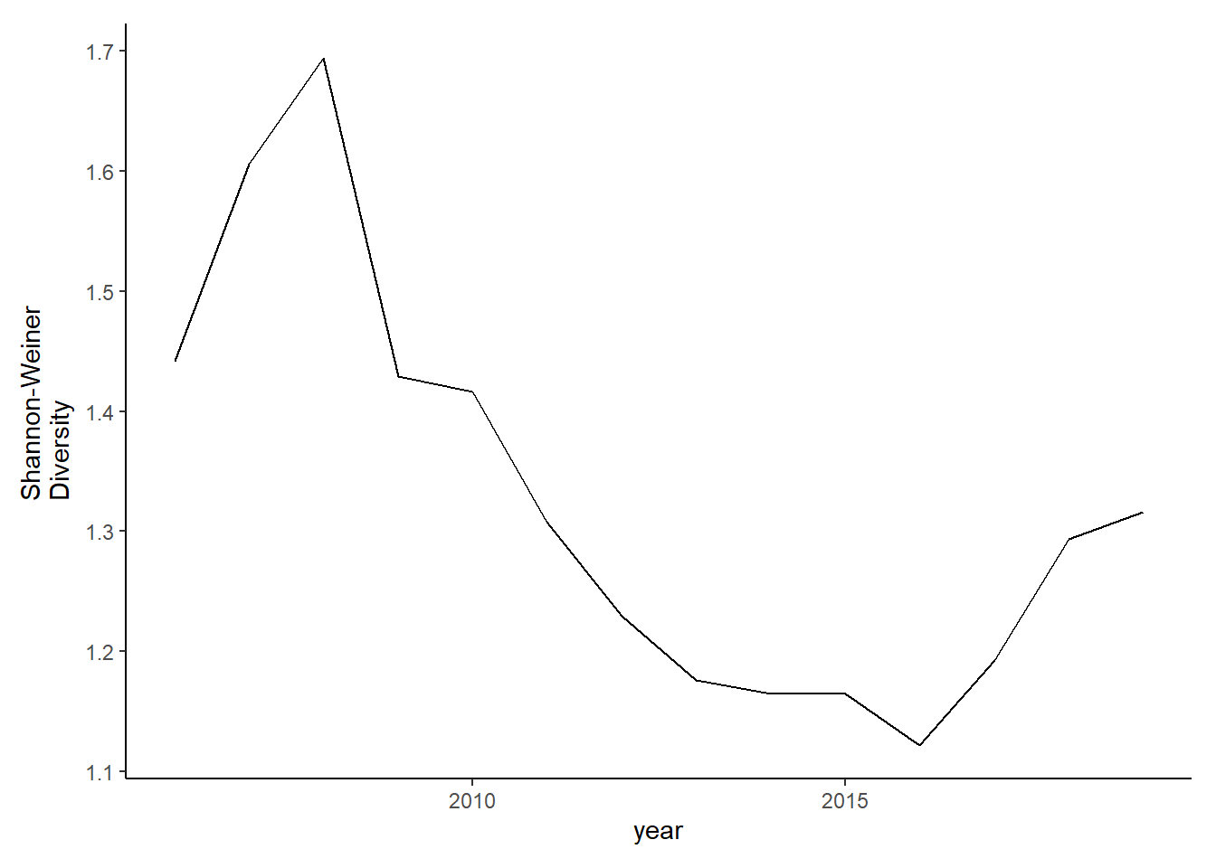
shannon2<-group_by(species_county_filter2, year,species)%>%
mutate(species_total=sum(total_weight))%>%
group_by(year)%>%
mutate(total=sum(species_total),prop=species_total/total)%>%
summarise(shannon=-1*(sum(prop*log(prop))))
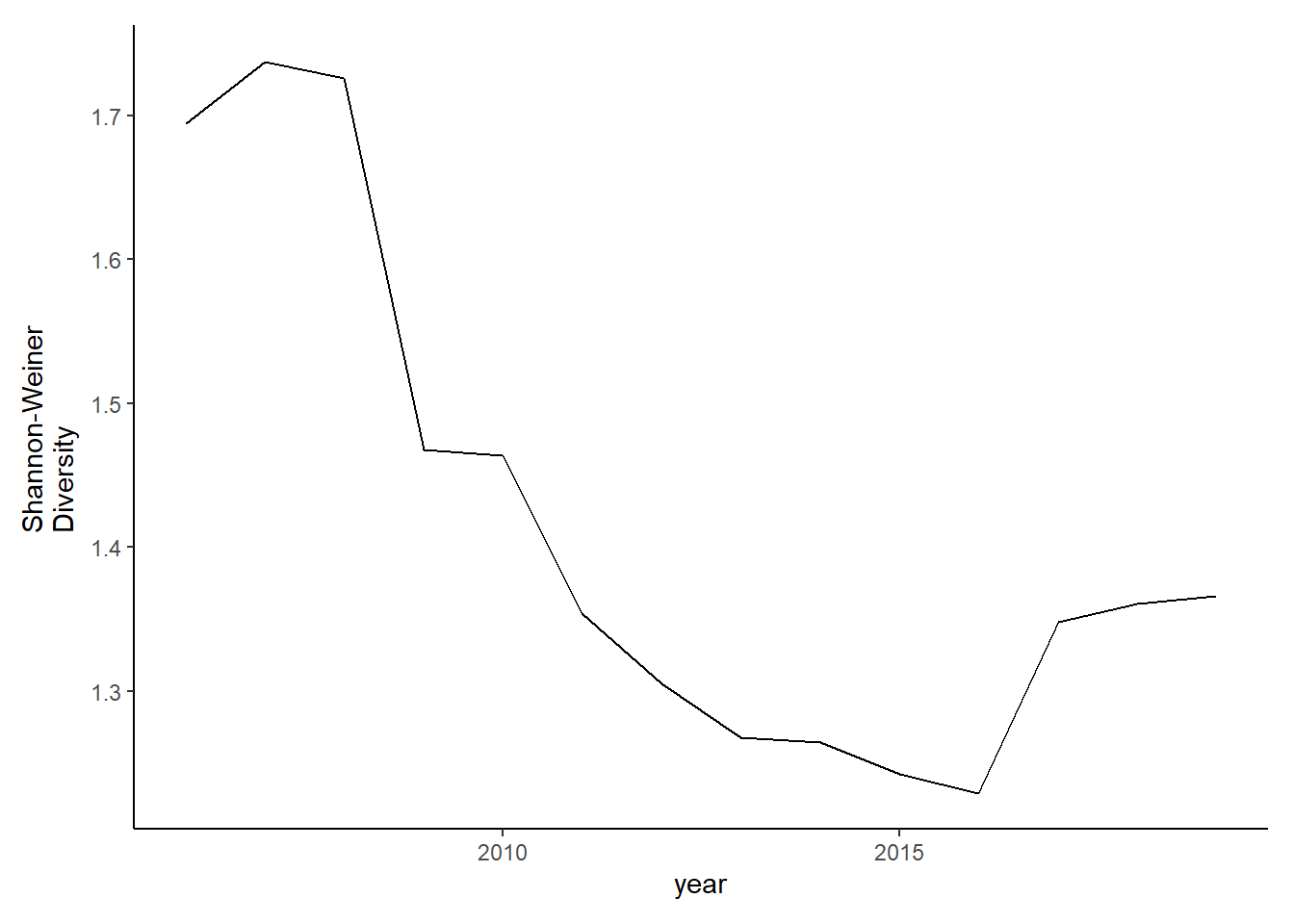
diversity2<-ggplot()+geom_line(data=subset(shannon2, year<2020), aes(year, shannon))+theme_classic()+ ylab(expression(paste("Shannon-Weiner\nDiversity")))+theme(plot.margin = margin(10, 10, 10, 20))
diversity2
Full data
shannon_full<-group_by(landings_full, year,species)%>%
  mutate(species_total=sum(total_weight))%>%
  group_by(year)%>%
  mutate(total=sum(species_total),prop=species_total/total)%>%
  summarise(shannon=-1*(sum(prop*log(prop))))

diversity_full<-ggplot()+geom_line(data=subset(shannon_full, year>2005), aes(year, shannon))+theme_classic()+ ylab(expression(paste("Shannon-Weiner\nDiversity")))+theme(plot.margin = margin(10, 10, 10, 20))

diversity_full
#filtered data
shannon_full2<-group_by(species_full_filter2, year,species)%>%
  mutate(species_total=sum(total_weight))%>%
  group_by(year)%>%
  mutate(total=sum(species_total),prop=species_total/total)%>%
  summarise(shannon=-1*(sum(prop*log(prop))))

diversity_full2<-ggplot()+geom_line(data=subset(shannon_full2, year>2005), aes(year, shannon))+theme_classic()+ ylab(expression(paste("Shannon-Weiner\nDiversity")))+theme(plot.margin = margin(10, 10, 10, 20))

diversity_full2
Simpson’s diversity and evenness
County specified data
simpson<-group_by(landings_total, year, county)%>%
mutate(total=sum(weight), prop=weight/total)%>%
summarise(simpson=1/(sum(prop^2)) )
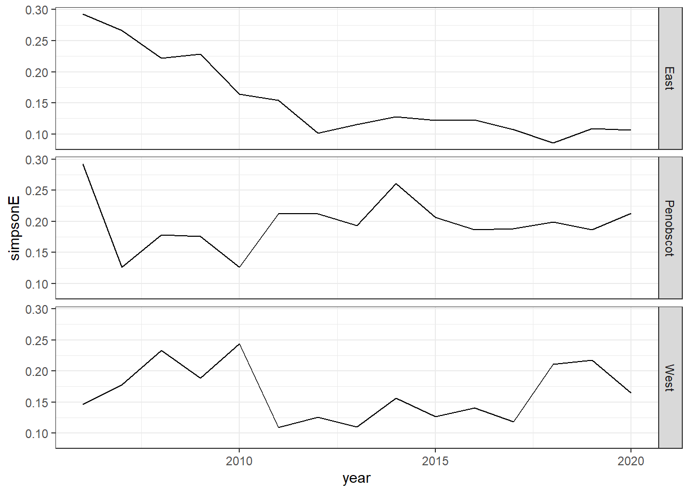
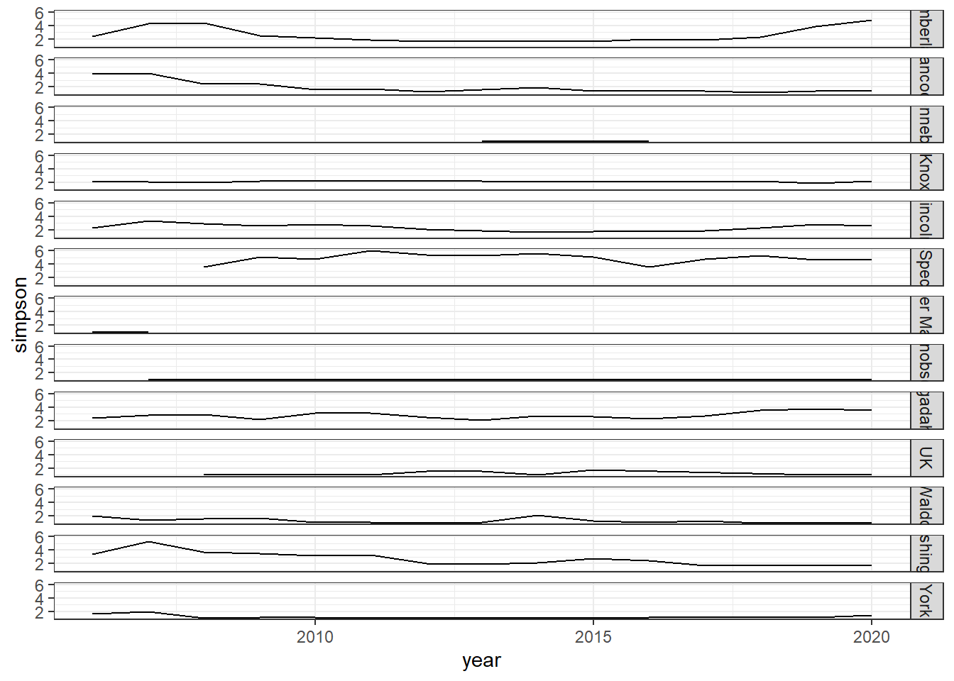
ggplot()+geom_line(data=simpson, aes(year, simpson))+
facet_grid(rows=vars(county))+theme_bw()
simpson<-group_by(landings_total, year,species)%>%
summarise(species_total=sum(weight))%>% #aggregate counties to get yearly species totals for all of Maine
group_by(year)%>%
mutate(richness=length(unique(species)))%>%
mutate(total=sum(species_total))%>%
mutate(prop=species_total/total)%>%
summarise(simpsonD=1/(sum(prop^2)),simpsonE=simpsonD*(1/richness))
#ggplot()+geom_line(data=simpson, aes(year, simpsonD))+theme_classic()
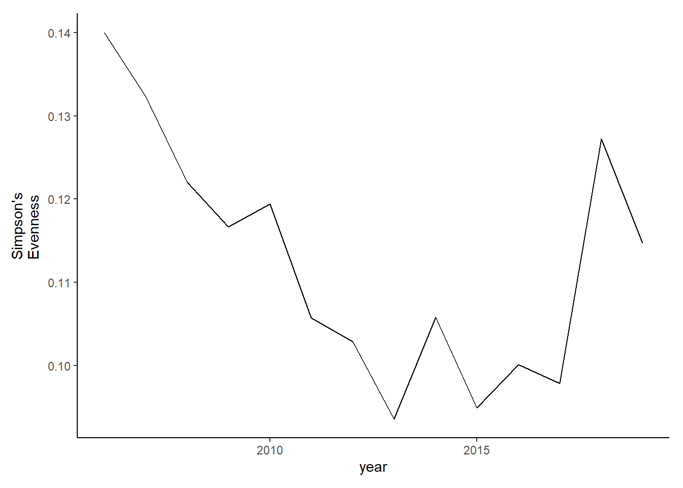
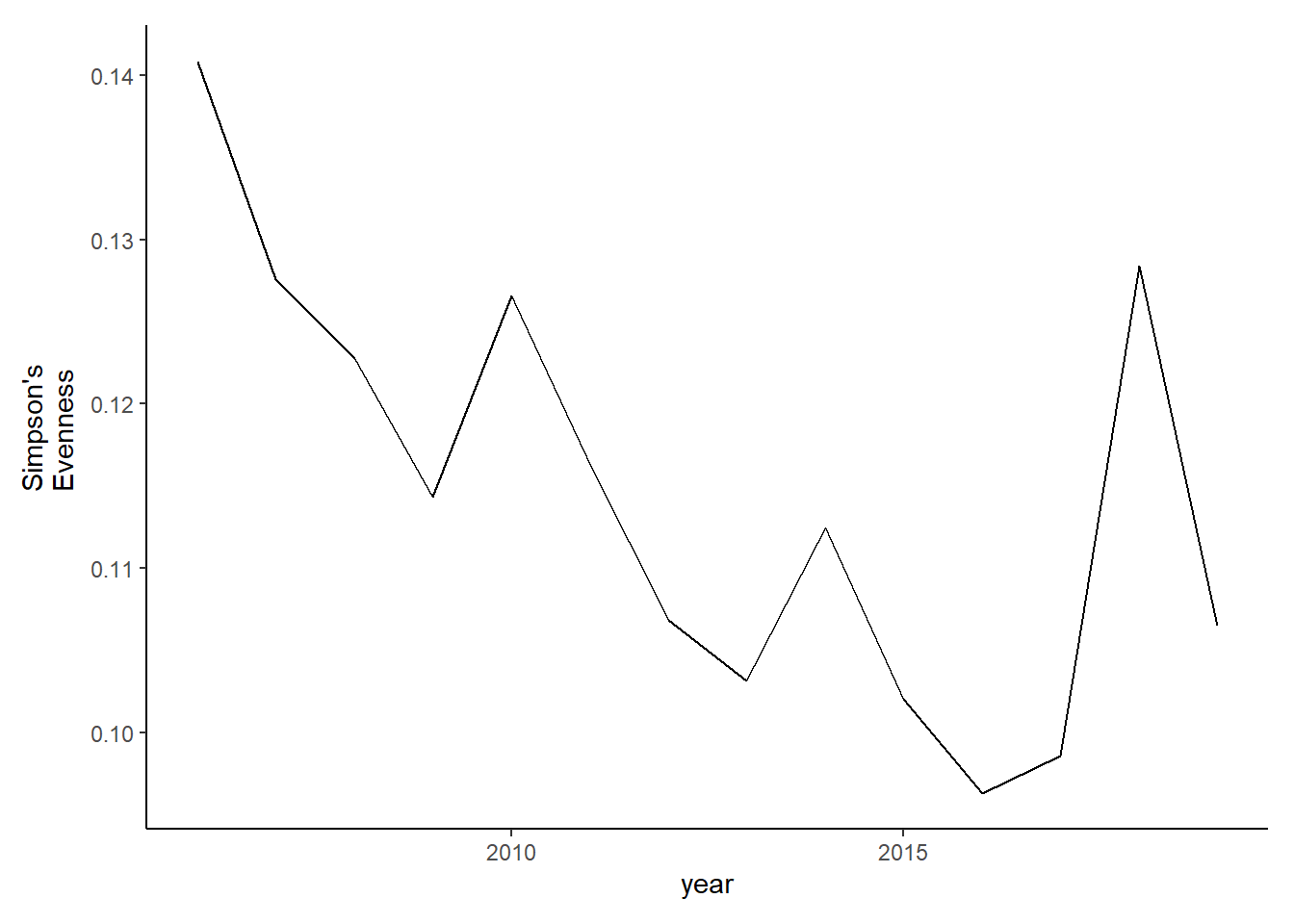
evenness<-ggplot()+geom_line(data=subset(simpson, year<2020), aes(year, simpsonE))+theme_classic()+ ylab(expression(paste("Simpson's\nEvenness")))+theme(plot.margin = margin(10, 10, 10, 20))
evenness
#filtered data
simpson2<-group_by(species_county_filter2, year,species)%>%
summarise(species_total=sum(total_weight))%>% #aggregate counties to get yearly species totals for all of Maine
group_by(year)%>%
mutate(richness=length(unique(species)))%>%
mutate(total=sum(species_total))%>%
mutate(prop=species_total/total)%>%
summarise(simpsonD=1/(sum(prop^2)),simpsonE=simpsonD*(1/richness))
#ggplot()+geom_line(data=simpson2, aes(year, simpsonD))+theme_classic()
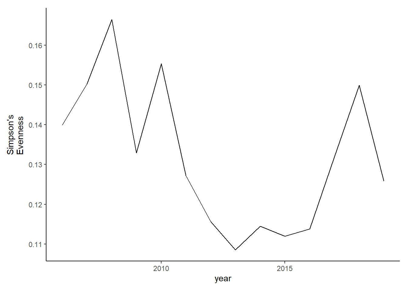
evenness2<-ggplot()+geom_line(data=subset(simpson2, year<2020), aes(year, simpsonE))+theme_classic()+ ylab(expression(paste("Simpson's\nEvenness")))+theme(plot.margin = margin(10, 10, 10, 20))
evenness2
Full data
simpson_full<-group_by(landings_full, year,species)%>%
summarise(species_total=sum(total_weight))%>% #aggregate counties to get yearly species totals for all of Maine
group_by(year)%>%
mutate(richness=length(unique(species)))%>%
mutate(total=sum(species_total))%>%
mutate(prop=species_total/total)%>%
summarise(simpsonD=1/(sum(prop^2)),simpsonE=simpsonD*(1/richness))
#ggplot()+geom_line(data=simpson_full, aes(year, simpsonD))+theme_classic()
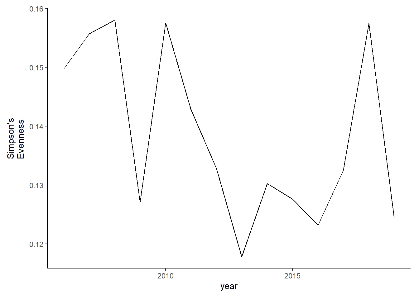
evenness_full<-ggplot()+geom_line(data=subset(simpson_full, year>2005), aes(year, simpsonE))+theme_classic()+ ylab(expression(paste("Simpson's\nEvenness")))+theme(plot.margin = margin(10, 10, 10, 20))
evenness_full
#filtered data
simpson_full2<-group_by(species_full_filter2, year,species)%>%
  summarise(species_total=sum(total_weight))%>% #aggregate counties to get yearly species totals for all of Maine
  group_by(year)%>%
  mutate(richness=length(unique(species)))%>%
  mutate(total=sum(species_total))%>%
  mutate(prop=species_total/total)%>%
  summarise(simpsonD=1/(sum(prop^2)),simpsonE=simpsonD*(1/richness))

#ggplot()+geom_line(data=simpson_full2, aes(year, simpsonD))+theme_classic()

evenness_full2<-ggplot()+geom_line(data=subset(simpson_full2, year>2005), aes(year, simpsonE))+theme_classic()+ ylab(expression(paste("Simpson's\nEvenness")))+theme(plot.margin = margin(10, 10, 10, 20))

evenness_full2
Average taxinomic distinctness
Country specified data
library(taxize)
library(purrr)
library(mgcv)

species<-read.csv(here("Data/species_landings.csv"))%>%
  filter(scientific.name!="")%>%
  filter(scientific.name!="Fucus vesiculosus")%>%
  rename(common_name=species, Species=scientific.name)


diff_species<-as.vector(unique(species$Species))
tax <- classification(diff_species, db = 'itis')
## ==  42 queries  ==============
## v  Found:  Gadus morhua
## v  Found:  Cancer irroratus
## v  Found:  Cancer borealis
## v  Found:  Brosme brosme
## v  Found:  Anguilla rostrata
## v  Found:  Glyptocephalus cynoglossus
## v  Found:  Pseudopleuronectes americanus
## v  Found:  Melanogrammus aeglefinus
## v  Found:  Urophycis tenuis
## v  Found:  Hippoglossus hippoglossus
## v  Found:  Clupea harengus
## v  Found:  Homarus americanus
## v  Found:  Lophius americanus
## v  Found:  Hippoglossoides platessoides
## v  Found:  Pollachius virens
## v  Found:  Sebastes fasciatus
## v  Found:  Placopecten magellanicus
## v  Found:  Pandalus borealis
## v  Found:  Anarhichas lupus
## v  Found:  Mytilus edulis
## v  Found:  Strongylocentrotus droebachiensis
## v  Found:  Crassostrea virginica
## v  Found:  Mercenaria mercenaria
## v  Found:  Limanda ferruginea
## v  Found:  Merluccius bilinearis
## v  Found:  Scomber scombrus
## v  Found:  Cucumaria frondosa
## v  Found:  Pomatomus saltatrix
## v  Found:  Brevoortia tyrannus
## v  Found:  Arctica islandica
## v  Found:  Ensis directus
## v  Found:  Squalus acanthias
## v  Found:  Myxine glutinosa
## v  Found:  Ostrea edulis
## v  Found:  Littorina littorea
## v  Found:  Loligo pealeii
## v  Found:  Thunnus thynnus
## v  Found:  Xiphias gladius
## v  Found:  Buccinum undatum
## v  Found:  Illex illecebrosus
## v  Found:  Thunnus obesus
## v  Found:  Spisula solidissima
## ==  Results  =================
##
## * Total: 42
## * Found: 42
## * Not Found: 0
info <- matrix(NA)
expand <- matrix(NA)
specific <- matrix(NA, nrow = length(diff_species), ncol=6)
for (i in 1:length(tax)){
info <- tax[[i]][c('name','rank')]
expand <- info[info$rank == 'phylum'| info$rank == 'class'| info$rank == 'order' | info$rank == 'family' | info$rank == 'genus' | info$rank == 'species',]
specific[i,] <- as.vector(expand$name)
}
colnames(specific) <- c("Phylum", "Class", "Order", "Family", "Genus", "Species")
phylo<-as.data.frame(specific)
merge<-left_join(species,phylo, by="Species")
landings_tax<-rename(landings_total, common_name=species)%>%
full_join(merge)%>%
filter(!is.na(Species))
landings_tax_groups<-group_by(landings_tax, year,Species)%>%
summarise(weight=sum(weight))%>%
mutate(indicator=cur_group_id())%>%
left_join(phylo)
hauls <- unique(landings_tax_groups$indicator)
N_hauls <- length(hauls) # number of hauls
N_species <- NULL #N species
sub_species <- NULL # N_species-1
total <- NULL #xixj
numerator <- NULL #wijxixj
x_y <- matrix(NA, nrow = 6, ncol = 6)
x <- NULL
y <- NULL
ident <- NULL
weight <- NULL #wij
count <- NULL
total_weight <- NULL
mean_weight <- NULL
weight_var <- NULL
delta <- NULL
delta_star <- NULL
delta_plus <- NULL
delta_var <- NULL
weight_var <- NULL
for (j in 1:N_hauls) {
diff_hauls <- landings_tax_groups[which(landings_tax_groups$indicator == j),] #subset unique hauls/functional groups
N_species[j] <- length(unique(diff_hauls$Species))# count the number of unique species in each haul (denominator)
sub_species[j] <- N_species[j]-1
diff <- unique(as.vector(diff_hauls$Species)) # name of each unique species
combos <- combn(diff, 2) # create combinations of each species/haul (for weight calc)
phylo <- as.matrix(subset(diff_hauls, select = c(Phylum,Class,Order,Family,Genus, Species))) # extract phylogenetic information only
unique_phylo <- uniquecombs(phylo) # subset by unique species information
unique_phylo <- as.data.frame(unique_phylo)
total <- NULL # reset the length for each haul because they will be different
weight <- NULL # reset
for (i in 1:ncol(combos)) { # for each unique combination count the number of each species
total[i] <- sum(diff_hauls$Species == combos[1,i]) * sum(diff_hauls$Species == combos[2,i]) #empty vector is always length 210
#total[i] <- diff_hauls[diff_hauls[,22] == combos[1,i],9] * diff_hauls[diff_hauls[,22] == combos[2,i],9]
x <- unique_phylo[unique_phylo$Species == combos[1,i],]
y <- unique_phylo[unique_phylo$Species == combos[2,i],]
x_y <- rbind(x,y)
for (k in 1:ncol(x_y)){ # for each combination calculate the weight value
ident[k] <- identical(as.vector(x_y[1,k]), as.vector(x_y[2,k])) # determine how much of phylogenetic information is the same
weight[i] <- sum(ident == "FALSE") # vector of weights
#mean_weight[i] <- mean(weight) #rep(mean(weight),length(weight))
numerator[j] <- sum(total*weight)
count[j] <- sum(total)
mean_weight[j] <- mean(weight)
total_weight[j] <- sum(weight)
weight_var[j] <- sum((weight- mean(weight))^2)
}
delta <- (2*numerator)/(N_species*sub_species)
delta_star <- numerator/(count)
delta_plus <- (2*total_weight)/(N_species*sub_species)
delta_var <- (2*weight_var)/(N_species*sub_species) #double check that this equation is correct
}
}
years<-2006:2020
delta<-as.data.frame(delta[1:15]) # taxonomic diversity
delta_star<-as.data.frame(delta_star[1:15]) # taxonomic distinctness
delta_plus<-as.data.frame(delta_plus[1:15]) # average taxonomic distinctness
delta_var<-as.data.frame(delta_var[1:15]) # variation in taxonomic distinctness
d<-bind_cols(years,delta, delta_star,delta_plus,delta_var)
colnames(d)<-c("year", "delta", "delta_star", "delta_plus","delta_var")
#write.csv(d, here("Data/tax_metrics.csv"))
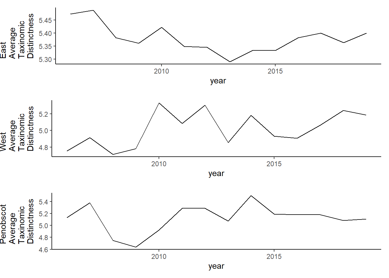
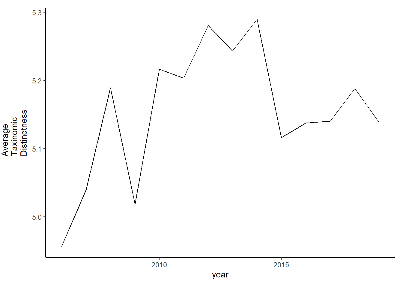
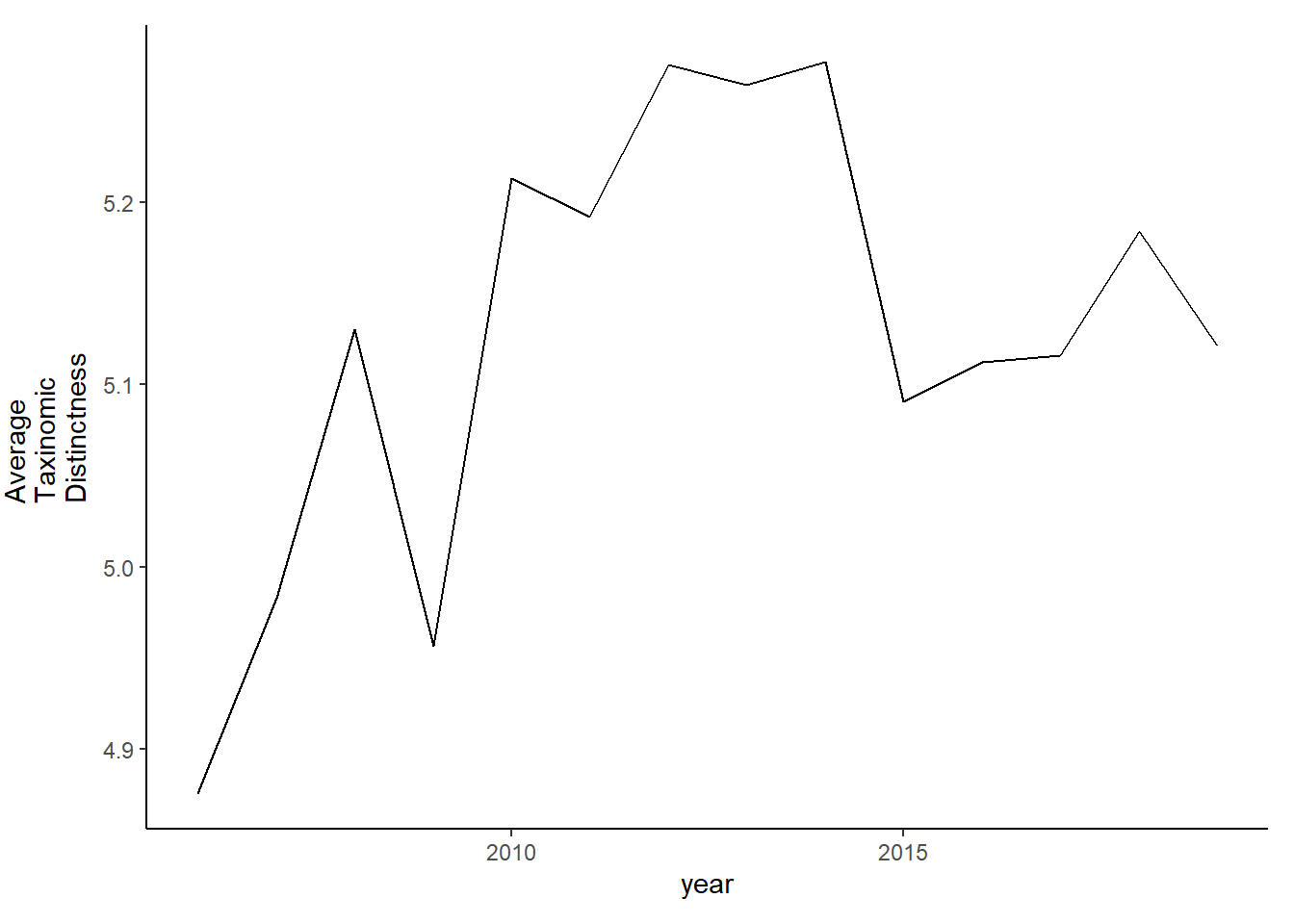
tax.distinct<-ggplot()+geom_line(data=subset(d, year<2020), aes(year, delta_plus))+theme_classic()+ylab(expression(paste("Average\nTaxinomic\nDistinctness")))+theme(plot.margin = margin(10, 10, 10, 25))
tax.distinct
With filtered data
species<-read.csv(here("Data/species_landings.csv"))%>%
  filter(scientific.name!="")%>%
  filter(scientific.name!="Fucus vesiculosus")%>%
  anti_join(remove_county)%>%
  rename(common_name=species, Species=scientific.name)


diff_species<-as.vector(unique(species$Species))
tax <- classification(diff_species, db = 'itis')
## ==  35 queries  ==============
## v  Found:  Gadus morhua
## v  Found:  Cancer irroratus
## v  Found:  Cancer borealis
## v  Found:  Brosme brosme
## v  Found:  Anguilla rostrata
## v  Found:  Glyptocephalus cynoglossus
## v  Found:  Pseudopleuronectes americanus
## v  Found:  Melanogrammus aeglefinus
## v  Found:  Urophycis tenuis
## v  Found:  Hippoglossus hippoglossus
## v  Found:  Clupea harengus
## v  Found:  Homarus americanus
## v  Found:  Lophius americanus
## v  Found:  Hippoglossoides platessoides
## v  Found:  Pollachius virens
## v  Found:  Sebastes fasciatus
## v  Found:  Placopecten magellanicus
## v  Found:  Pandalus borealis
## v  Found:  Anarhichas lupus
## v  Found:  Mytilus edulis
## v  Found:  Strongylocentrotus droebachiensis
## v  Found:  Mercenaria mercenaria
## v  Found:  Limanda ferruginea
## v  Found:  Merluccius bilinearis
## v  Found:  Scomber scombrus
## v  Found:  Cucumaria frondosa
## v  Found:  Pomatomus saltatrix
## v  Found:  Brevoortia tyrannus
## v  Found:  Arctica islandica
## v  Found:  Ensis directus
## v  Found:  Squalus acanthias
## v  Found:  Ostrea edulis
## v  Found:  Loligo pealeii
## v  Found:  Buccinum undatum
## v  Found:  Illex illecebrosus
## ==  Results  =================
##
## * Total: 35
## * Found: 35
## * Not Found: 0
info <- matrix(NA)
expand <- matrix(NA)
specific <- matrix(NA, nrow = length(diff_species), ncol=6)
for (i in 1:length(tax)){
info <- tax[[i]][c('name','rank')]
expand <- info[info$rank == 'phylum'| info$rank == 'class'| info$rank == 'order' | info$rank == 'family' | info$rank == 'genus' | info$rank == 'species',]
specific[i,] <- as.vector(expand$name)
}
colnames(specific) <- c("Phylum", "Class", "Order", "Family", "Genus", "Species")
phylo<-as.data.frame(specific)
merge<-left_join(species,phylo, by="Species")
landings_tax<-rename(landings_total, common_name=species)%>%
full_join(merge)%>%
filter(!is.na(Species))
landings_tax_groups<-group_by(landings_tax, year,Species)%>%
summarise(weight=sum(weight))%>%
mutate(indicator=cur_group_id())%>%
left_join(phylo)
hauls <- unique(landings_tax_groups$indicator)
N_hauls <- length(hauls) # number of hauls
N_species <- NULL #N species
sub_species <- NULL # N_species-1
total <- NULL #xixj
numerator <- NULL #wijxixj
x_y <- matrix(NA, nrow = 6, ncol = 6)
x <- NULL
y <- NULL
ident <- NULL
weight <- NULL #wij
count <- NULL
total_weight <- NULL
mean_weight <- NULL
weight_var <- NULL
delta <- NULL
delta_star <- NULL
delta_plus <- NULL
delta_var <- NULL
weight_var <- NULL
for (j in 1:N_hauls) {
diff_hauls <- landings_tax_groups[which(landings_tax_groups$indicator == j),] #subset unique hauls/functional groups
N_species[j] <- length(unique(diff_hauls$Species))# count the number of unique species in each haul (denominator)
sub_species[j] <- N_species[j]-1
diff <- unique(as.vector(diff_hauls$Species)) # name of each unique species
combos <- combn(diff, 2) # create combinations of each species/haul (for weight calc)
phylo <- as.matrix(subset(diff_hauls, select = c(Phylum,Class,Order,Family,Genus, Species))) # extract phylogenetic information only
unique_phylo <- uniquecombs(phylo) # subset by unique species information
unique_phylo <- as.data.frame(unique_phylo)
total <- NULL # reset the length for each haul because they will be different
weight <- NULL # reset
for (i in 1:ncol(combos)) { # for each unique combination count the number of each species
total[i] <- sum(diff_hauls$Species == combos[1,i]) * sum(diff_hauls$Species == combos[2,i]) #empty vector is always length 210
#total[i] <- diff_hauls[diff_hauls[,22] == combos[1,i],9] * diff_hauls[diff_hauls[,22] == combos[2,i],9]
x <- unique_phylo[unique_phylo$Species == combos[1,i],]
y <- unique_phylo[unique_phylo$Species == combos[2,i],]
x_y <- rbind(x,y)
for (k in 1:ncol(x_y)){ # for each combination calculate the weight value
ident[k] <- identical(as.vector(x_y[1,k]), as.vector(x_y[2,k])) # determine how much of phylogenetic information is the same
weight[i] <- sum(ident == "FALSE") # vector of weights
#mean_weight[i] <- mean(weight) #rep(mean(weight),length(weight))
numerator[j] <- sum(total*weight)
count[j] <- sum(total)
mean_weight[j] <- mean(weight)
total_weight[j] <- sum(weight)
weight_var[j] <- sum((weight- mean(weight))^2)
}
delta <- (2*numerator)/(N_species*sub_species)
delta_star <- numerator/(count)
delta_plus <- (2*total_weight)/(N_species*sub_species)
delta_var <- (2*weight_var)/(N_species*sub_species) #double check that this equation is correct
}
}
years<-2006:2020
delta<-as.data.frame(delta[1:15]) # taxonomic diversity
delta_star<-as.data.frame(delta_star[1:15]) # taxonomic distinctness
delta_plus<-as.data.frame(delta_plus[1:15]) # average taxonomic distinctness
delta_var<-as.data.frame(delta_var[1:15]) # variation in taxonomic distinctness
d2<-bind_cols(years,delta, delta_star,delta_plus,delta_var)
colnames(d2)<-c("year", "delta", "delta_star", "delta_plus","delta_var")
#write.csv(d, here("Data/tax_metrics.csv"))
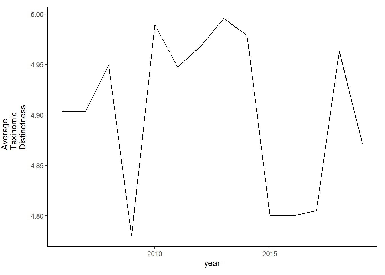
tax.distinct2<-ggplot()+geom_line(data=subset(d2, year<2020), aes(year, delta_plus))+theme_classic()+ylab(expression(paste("Average\nTaxinomic\nDistinctness")))+theme(plot.margin = margin(10, 10, 10, 25))
tax.distinct2
Full data
unique<-as.data.frame(unique(species_full$species))%>%
  rename(common_name="unique(species_full$species)")

species2<-read.csv(here("Data/species_landings.csv"))%>%
  filter(scientific.name!="Fucus vesiculosus")%>%
  anti_join(remove_full)%>%
  rename(common_name=species, Species=scientific.name)%>%
  right_join(unique)

species2$Species[species2$common_name=="Alewife"]<-"Alosa pseudoharengus"
species2$Species[species2$common_name=="Salmon Atlantic"]<-"Salmo salar"

species<-species2%>%
  filter(Species!="NA")%>%
  filter(Species!="")

diff_species<-as.vector(unique(species$Species))
tax <- classification(diff_species, db = 'itis')
## ==  27 queries  ==============
## v  Found:  Gadus morhua
## v  Found:  Brosme brosme
## v  Found:  Glyptocephalus cynoglossus
## v  Found:  Pseudopleuronectes americanus
## v  Found:  Melanogrammus aeglefinus
## v  Found:  Urophycis tenuis
## v  Found:  Hippoglossus hippoglossus
## v  Found:  Clupea harengus
## v  Found:  Homarus americanus
## v  Found:  Lophius americanus
## v  Found:  Hippoglossoides platessoides
## v  Found:  Pollachius virens
## v  Found:  Sebastes fasciatus
## v  Found:  Placopecten magellanicus
## v  Found:  Pandalus borealis
## v  Found:  Anarhichas lupus
## v  Found:  Mytilus edulis
## v  Found:  Strongylocentrotus droebachiensis
## v  Found:  Mercenaria mercenaria
## v  Found:  Limanda ferruginea
## v  Found:  Merluccius bilinearis
## v  Found:  Scomber scombrus
## v  Found:  Cucumaria frondosa
## v  Found:  Brevoortia tyrannus
## v  Found:  Arctica islandica
## v  Found:  Alosa pseudoharengus
## v  Found:  Salmo salar
## ==  Results  =================
##
## * Total: 27
## * Found: 27
## * Not Found: 0
info <- matrix(NA)
expand <- matrix(NA)
specific <- matrix(NA, nrow = length(diff_species), ncol=6)


for (i in 1:length(tax)){
info <- tax[[i]][c('name','rank')]
expand <- info[info$rank == 'phylum'| info$rank == 'class'| info$rank == 'order' | info$rank == 'family' | info$rank == 'genus' | info$rank == 'species',]
specific[i,] <- as.vector(expand$name)

}
colnames(specific) <- c("Phylum", "Class", "Order", "Family", "Genus", "Species")
phylo<-as.data.frame(specific)

merge<-left_join(species,phylo, by="Species")

landings_tax<-rename(landings_full, common_name=species)%>%
  full_join(merge)%>%
  filter(!is.na(Species))

landings_tax_groups<-group_by(landings_tax, year,Species)%>%
  summarise(weight=sum(total_weight))%>%
  mutate(indicator=cur_group_id())%>%
  left_join(phylo)

hauls <- unique(landings_tax_groups$indicator)
N_hauls <- length(hauls) # number of hauls
N_species <- NULL #N species
sub_species <- NULL # N_species-1
total <- NULL  #xixj
numerator <- NULL #wijxixj
x_y <- matrix(NA, nrow = 6, ncol = 6)
x <- NULL
y <- NULL
ident <- NULL
weight <- NULL #wij
count <- NULL
total_weight <- NULL
mean_weight <- NULL
weight_var <- NULL
delta <- NULL
delta_star <- NULL
delta_plus <- NULL
delta_var <- NULL
weight_var <- NULL

for (j in 1:N_hauls) {
diff_hauls <- landings_tax_groups[which(landings_tax_groups$indicator == j),] #subset unique hauls/functional groups
N_species[j] <- length(unique(diff_hauls$Species))# count the number of unique species in each haul (denominator)
sub_species[j] <- N_species[j]-1
diff <- unique(as.vector(diff_hauls$Species)) # name of each unique species
combos <- combn(diff, 2) # create combinations of each species/haul (for weight calc)

phylo <- as.matrix(subset(diff_hauls, select = c(Phylum,Class,Order,Family,Genus, Species))) # extract phylogenetic information only
unique_phylo <- uniquecombs(phylo) # subset by unique species information
unique_phylo <- as.data.frame(unique_phylo)

total <- NULL  # reset the length for each haul because they will be different
weight <- NULL # reset

for (i in 1:ncol(combos)) { # for each unique combination count the number of each species
  total[i] <- sum(diff_hauls$Species == combos[1,i]) * sum(diff_hauls$Species == combos[2,i]) #empty vector is always length 210
  #total[i] <- diff_hauls[diff_hauls[,22] == combos[1,i],9] * diff_hauls[diff_hauls[,22] == combos[2,i],9]
  x <- unique_phylo[unique_phylo$Species == combos[1,i],]
  y <- unique_phylo[unique_phylo$Species == combos[2,i],]
  x_y <- rbind(x,y)

  for (k in 1:ncol(x_y)){ # for each combination calculate the weight value
    ident[k] <- identical(as.vector(x_y[1,k]), as.vector(x_y[2,k])) # determine how much of phylogenetic information is the same
    weight[i] <- sum(ident == "FALSE") # vector of weights
    #mean_weight[i] <- mean(weight) #rep(mean(weight),length(weight))
    numerator[j] <- sum(total*weight)
    count[j] <- sum(total)
    mean_weight[j] <- mean(weight)
    total_weight[j] <- sum(weight)
    weight_var[j] <- sum((weight- mean(weight))^2)
  }
  delta <- (2*numerator)/(N_species*sub_species)
  delta_star <- numerator/(count)
  delta_plus <- (2*total_weight)/(N_species*sub_species)
  delta_var <- (2*weight_var)/(N_species*sub_species) #double check that this equation is correct
}
}
years<-1950:2019
delta<-as.data.frame(delta[1:70]) # taxonomic diversity
delta_star<-as.data.frame(delta_star[1:70]) # taxonomic distinctness
delta_plus<-as.data.frame(delta_plus[1:70]) # average taxonomic distinctness
delta_var<-as.data.frame(delta_var[1:70]) # variation in taxonomic distinctness

d_full<-bind_cols(years,delta, delta_star,delta_plus,delta_var)
colnames(d_full)<-c("year", "delta", "delta_star", "delta_plus","delta_var")

#write.csv(d_full, here("Data/tax_metrics_full.csv"))

tax.distinct_full<-ggplot()+geom_line(data=subset(d_full, year>2005), aes(year, delta_plus))+theme_classic()+ylab(expression(paste("Average\nTaxinomic\nDistinctness")))+theme(plot.margin = margin(10, 10, 10, 25))
                                                                      tax.distinct_full
filtered data
library(taxize)
library(purrr)
library(mgcv)

unique<-as.data.frame(unique(species_full_filter2$species))%>%
  rename(common_name="unique(species_full_filter2$species)")

species2<-read.csv(here("Data/species_landings.csv"))%>%
  filter(scientific.name!="Fucus vesiculosus")%>%
  rename(common_name=species, Species=scientific.name)%>%
  right_join(unique)

species2$Species[species2$common_name=="Alewife"]<-"Alosa pseudoharengus"

species<-species2%>%
  filter(Species!="NA")%>%
  filter(Species!="")

diff_species<-as.vector(unique(species$Species))
tax <- classification(diff_species, db = 'itis')
## ==  26 queries  ==============
## v  Found:  Gadus morhua
## v  Found:  Brosme brosme
## v  Found:  Glyptocephalus cynoglossus
## v  Found:  Pseudopleuronectes americanus
## v  Found:  Melanogrammus aeglefinus
## v  Found:  Urophycis tenuis
## v  Found:  Hippoglossus hippoglossus
## v  Found:  Clupea harengus
## v  Found:  Homarus americanus
## v  Found:  Lophius americanus
## v  Found:  Hippoglossoides platessoides
## v  Found:  Pollachius virens
## v  Found:  Sebastes fasciatus
## v  Found:  Placopecten magellanicus
## v  Found:  Pandalus borealis
## v  Found:  Anarhichas lupus
## v  Found:  Mytilus edulis
## v  Found:  Strongylocentrotus droebachiensis
## v  Found:  Mercenaria mercenaria
## v  Found:  Limanda ferruginea
## v  Found:  Merluccius bilinearis
## v  Found:  Scomber scombrus
## v  Found:  Cucumaria frondosa
## v  Found:  Brevoortia tyrannus
## v  Found:  Arctica islandica
## v  Found:  Alosa pseudoharengus
## ==  Results  =================
##
## * Total: 26
## * Found: 26
## * Not Found: 0
info <- matrix(NA)
expand <- matrix(NA)
specific <- matrix(NA, nrow = length(diff_species), ncol=6)
for (i in 1:length(tax)){
info <- tax[[i]][c('name','rank')]
expand <- info[info$rank == 'phylum'| info$rank == 'class'| info$rank == 'order' | info$rank == 'family' | info$rank == 'genus' | info$rank == 'species',]
specific[i,] <- as.vector(expand$name)
}
colnames(specific) <- c("Phylum", "Class", "Order", "Family", "Genus", "Species")
phylo<-as.data.frame(specific)
merge<-left_join(species,phylo, by="Species")
landings_tax<-rename(landings_full, common_name=species)%>%
full_join(merge)%>%
filter(!is.na(Species))
landings_tax_groups<-group_by(landings_tax, year,Species)%>%
summarise(weight=sum(total_weight))%>%
mutate(indicator=cur_group_id())%>%
left_join(phylo)
hauls <- unique(landings_tax_groups$indicator)
N_hauls <- length(hauls) # number of hauls
N_species <- NULL #N species
sub_species <- NULL # N_species-1
total <- NULL #xixj
numerator <- NULL #wijxixj
x_y <- matrix(NA, nrow = 6, ncol = 6)
x <- NULL
y <- NULL
ident <- NULL
weight <- NULL #wij
count <- NULL
total_weight <- NULL
mean_weight <- NULL
weight_var <- NULL
delta <- NULL
delta_star <- NULL
delta_plus <- NULL
delta_var <- NULL
weight_var <- NULL
for (j in 1:N_hauls) {
diff_hauls <- landings_tax_groups[which(landings_tax_groups$indicator == j),] #subset unique hauls/functional groups
N_species[j] <- length(unique(diff_hauls$Species))# count the number of unique species in each haul (denominator)
sub_species[j] <- N_species[j]-1
diff <- unique(as.vector(diff_hauls$Species)) # name of each unique species
combos <- combn(diff, 2) # create combinations of each species/haul (for weight calc)
phylo <- as.matrix(subset(diff_hauls, select = c(Phylum,Class,Order,Family,Genus, Species))) # extract phylogenetic information only
unique_phylo <- uniquecombs(phylo) # subset by unique species information
unique_phylo <- as.data.frame(unique_phylo)
total <- NULL # reset the length for each haul because they will be different
weight <- NULL # reset
for (i in 1:ncol(combos)) { # for each unique combination count the number of each species
total[i] <- sum(diff_hauls$Species == combos[1,i]) * sum(diff_hauls$Species == combos[2,i]) #empty vector is always length 210
#total[i] <- diff_hauls[diff_hauls[,22] == combos[1,i],9] * diff_hauls[diff_hauls[,22] == combos[2,i],9]
x <- unique_phylo[unique_phylo$Species == combos[1,i],]
y <- unique_phylo[unique_phylo$Species == combos[2,i],]
x_y <- rbind(x,y)
for (k in 1:ncol(x_y)){ # for each combination calculate the weight value
ident[k] <- identical(as.vector(x_y[1,k]), as.vector(x_y[2,k])) # determine how much of phylogenetic information is the same
weight[i] <- sum(ident == "FALSE") # vector of weights
#mean_weight[i] <- mean(weight) #rep(mean(weight),length(weight))
numerator[j] <- sum(total*weight)
count[j] <- sum(total)
mean_weight[j] <- mean(weight)
total_weight[j] <- sum(weight)
weight_var[j] <- sum((weight- mean(weight))^2)
}
delta <- (2*numerator)/(N_species*sub_species)
delta_star <- numerator/(count)
delta_plus <- (2*total_weight)/(N_species*sub_species)
delta_var <- (2*weight_var)/(N_species*sub_species) #double check that this equation is correct
}
}
years<-1950:2019
delta<-as.data.frame(delta[1:70]) # taxonomic diversity
delta_star<-as.data.frame(delta_star[1:70]) # taxonomic distinctness
delta_plus<-as.data.frame(delta_plus[1:70]) # average taxonomic distinctness
delta_var<-as.data.frame(delta_var[1:70]) # variation in taxonomic distinctness
d_full2<-bind_cols(years,delta, delta_star,delta_plus,delta_var)
colnames(d_full2)<-c("year", "delta", "delta_star", "delta_plus","delta_var")
#write.csv(d_full, here("Data/tax_metrics_full.csv"))
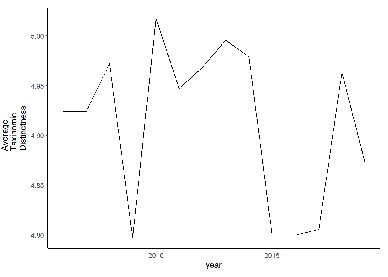
tax.distinct_full2<-ggplot()+geom_line(data=subset(d_full2, year>2005), aes(year, delta_plus))+theme_classic()+ylab(expression(paste("Average\nTaxinomic\nDistinctness")))+theme(plot.margin = margin(10, 10, 10, 25))
tax.distinct_full2
Combo plot
County specified data
library(reshape2)
library(gridExtra)
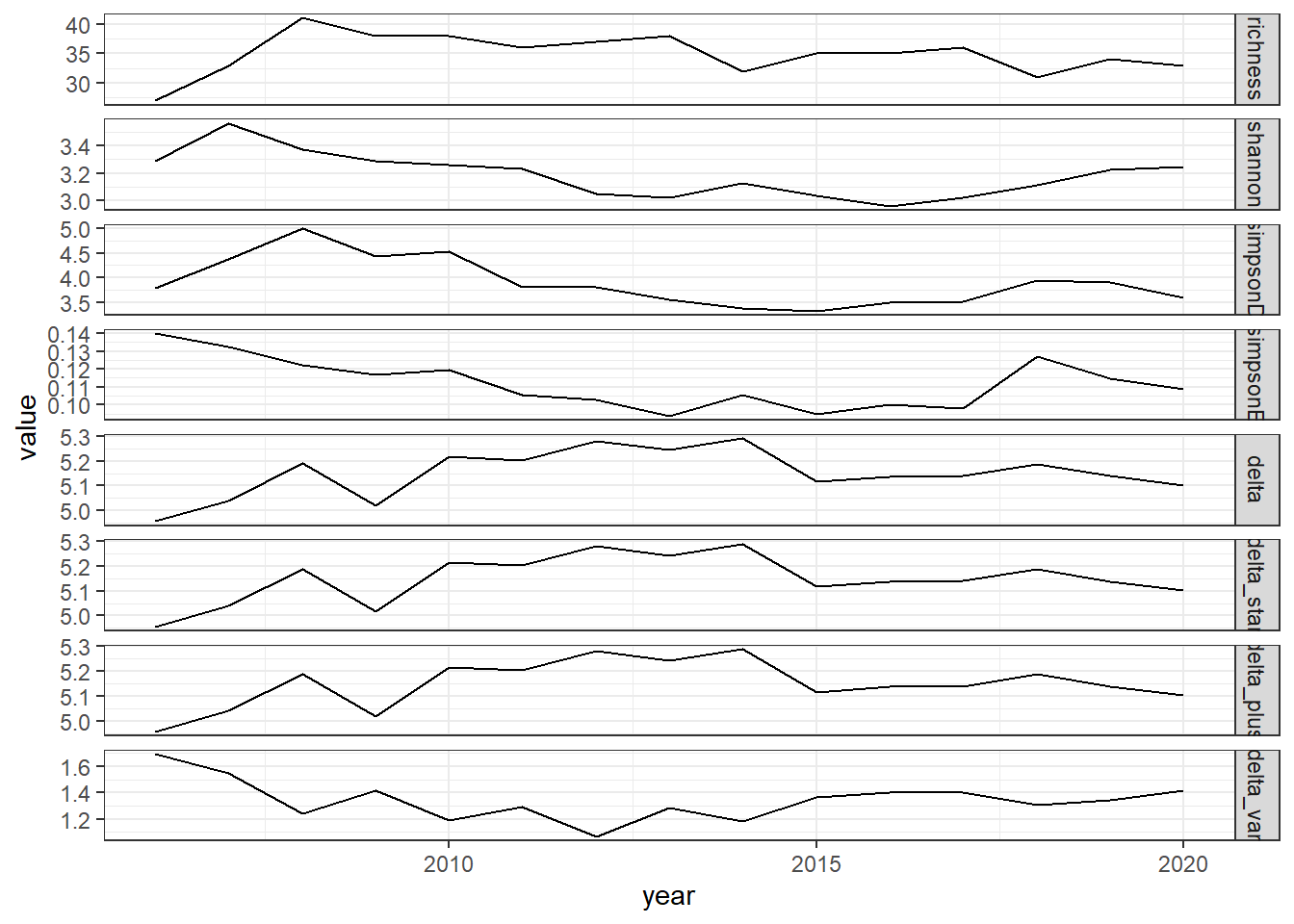
all_metrics<-full_join(richness,shannon, by="year")%>%
full_join(simpson)%>%
full_join(d)
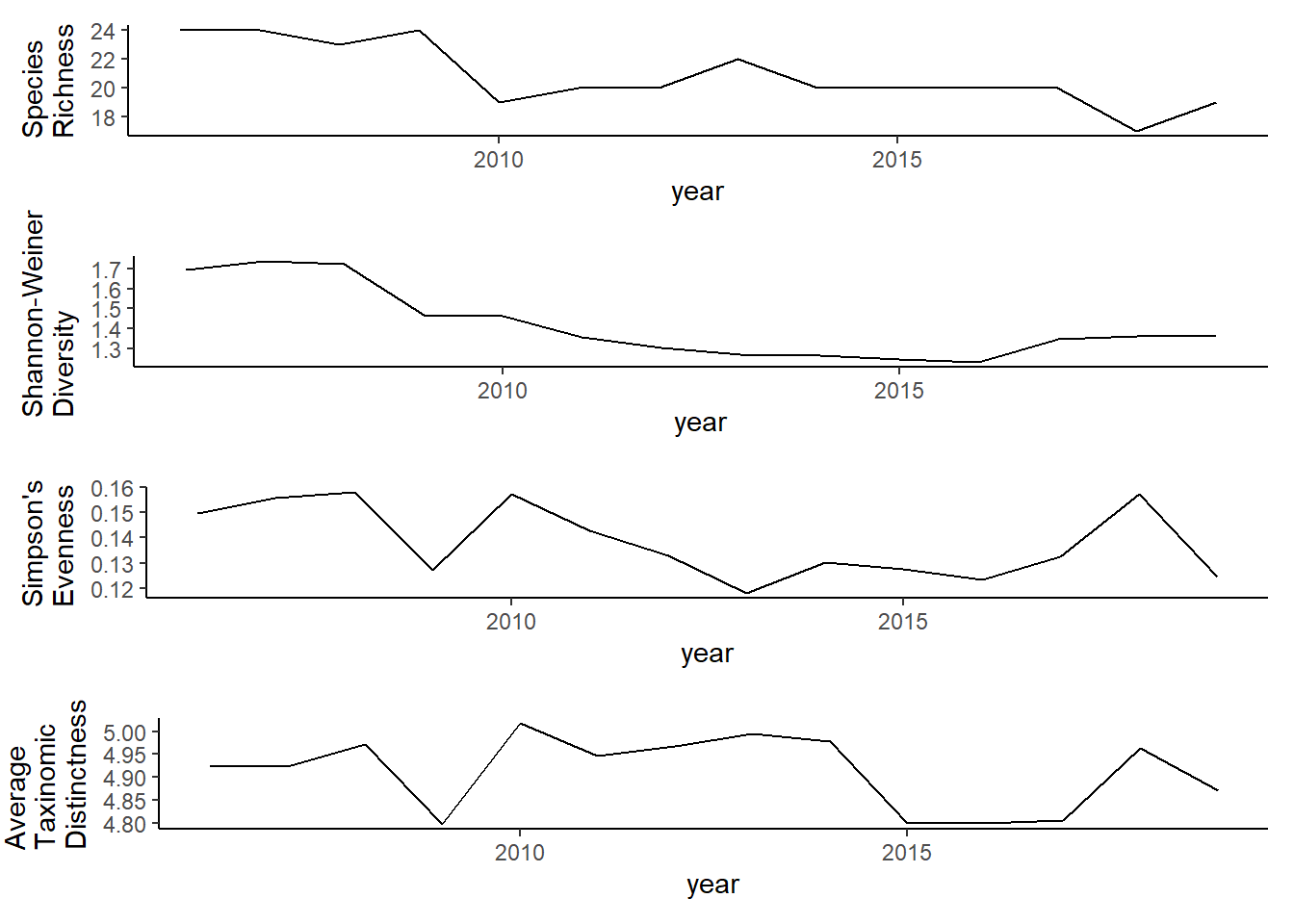
all_melt<-melt(all_metrics, id="year")
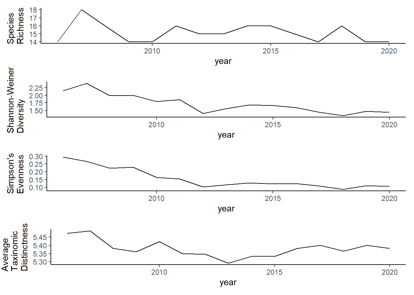
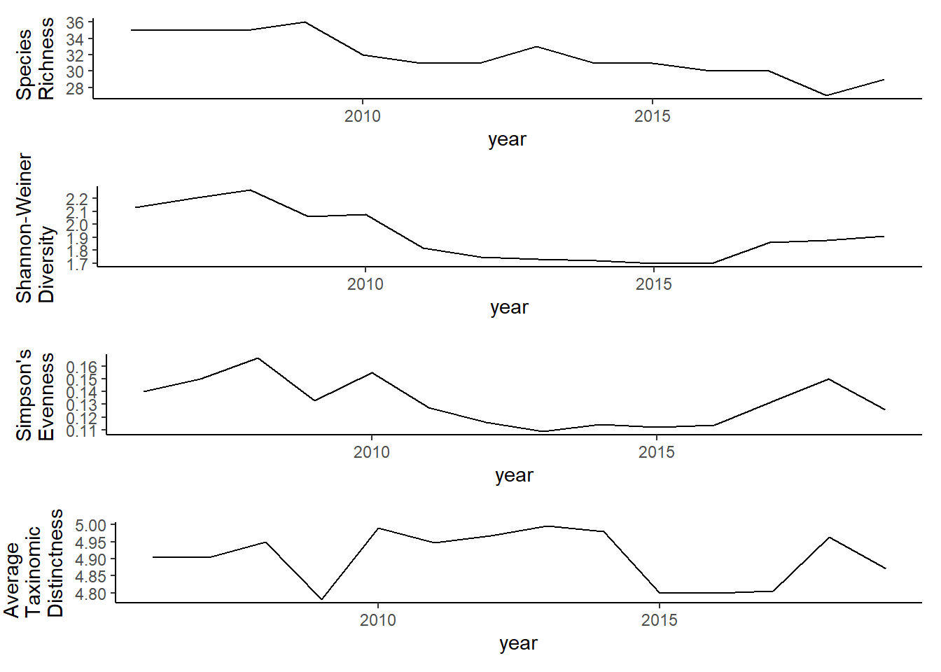
ggplot()+geom_line(data=all_melt, aes(year,value))+facet_grid(rows = vars(variable), scales="free")+theme_bw()
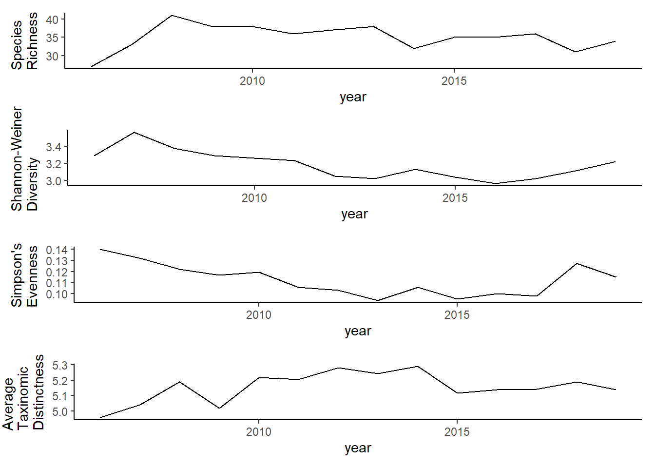
grid.arrange(rich, diversity, evenness,tax.distinct, nrow=4)
#filtered
all_metrics2<-full_join(richness2,shannon2, by="year")%>%
  full_join(simpson2)%>%
  full_join(d2)

all_melt2<-melt(all_metrics2, id="year")

ggplot()+geom_line(data=all_melt2, aes(year,value))+facet_grid(rows = vars(variable), scales="free")+theme_bw()
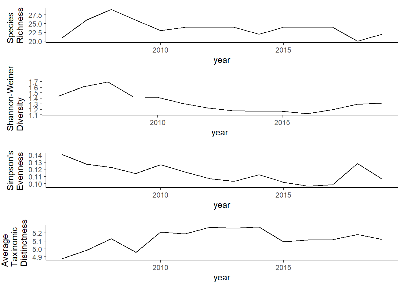
grid.arrange(rich2, diversity2, evenness2,tax.distinct2, nrow=4)
Full data
library(reshape2)
library(gridExtra)
all_metrics_full<-full_join(richness_full,shannon_full, by="year")%>%
full_join(simpson_full)%>%
full_join(d_full)
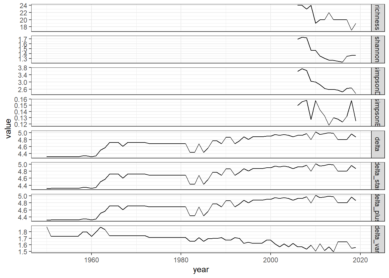
all_melt_full<-melt(all_metrics_full, id="year")
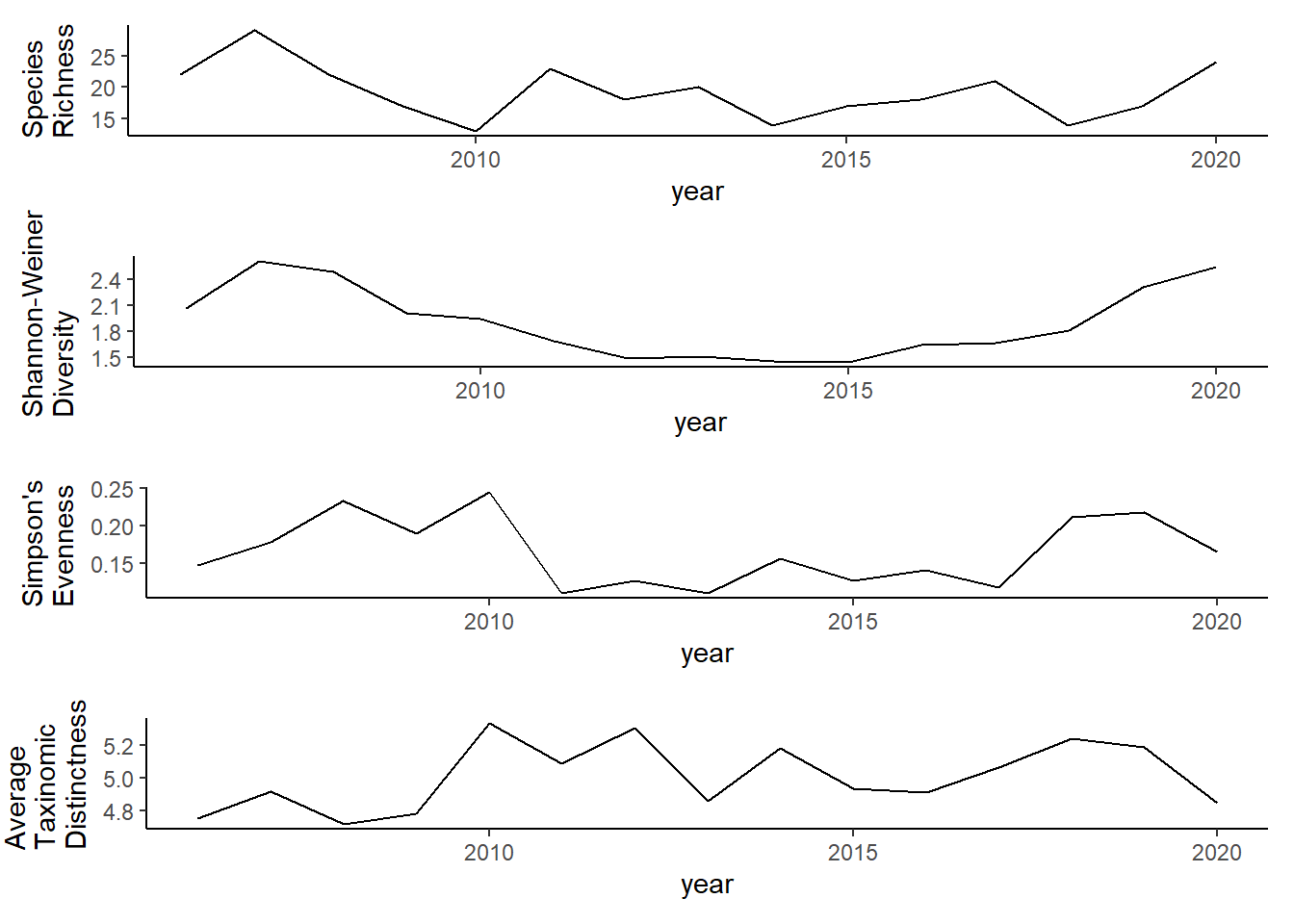
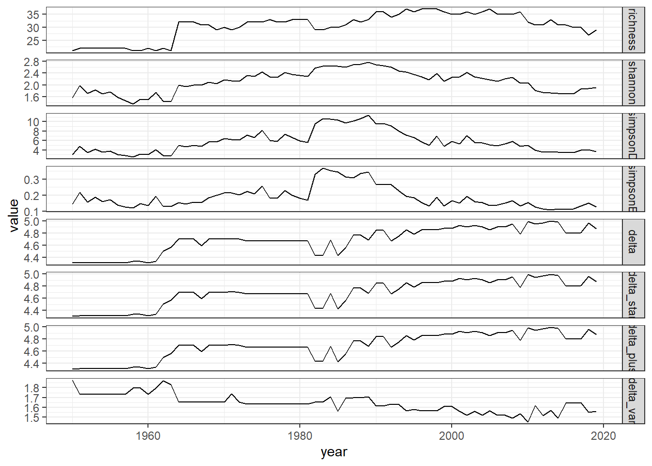
ggplot()+geom_line(data=all_melt_full, aes(year,value))+facet_grid(rows = vars(variable), scales="free")+theme_bw()
grid.arrange(rich_full, diversity_full, evenness_full,tax.distinct_full, nrow=4)
#filtered data
all_metrics_full2<-full_join(richness_full2,shannon_full2, by="year")%>%
full_join(simpson_full2)%>%
full_join(d_full2)
all_melt_full2<-melt(all_metrics_full2, id="year")
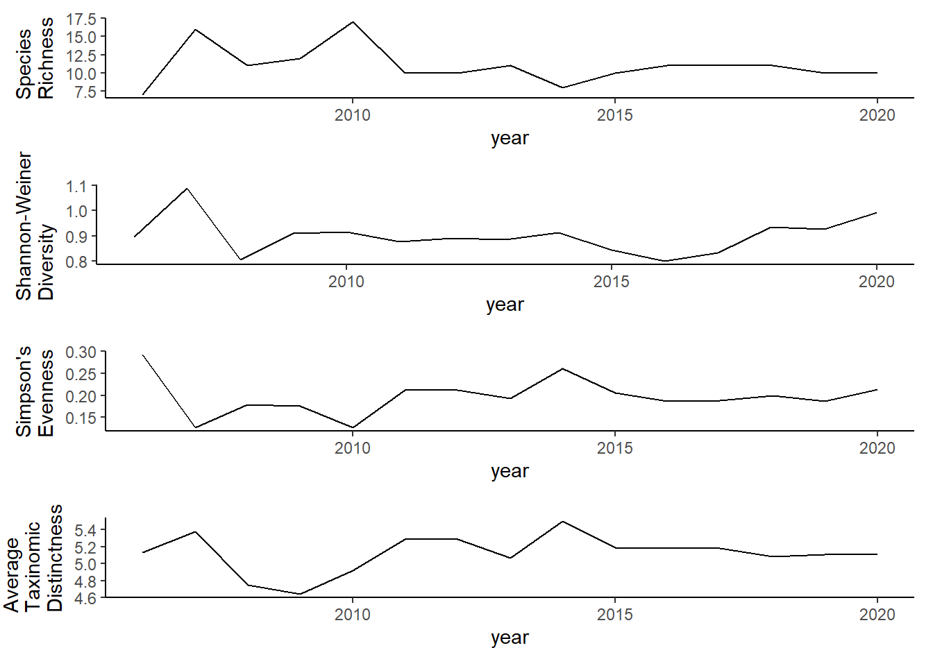
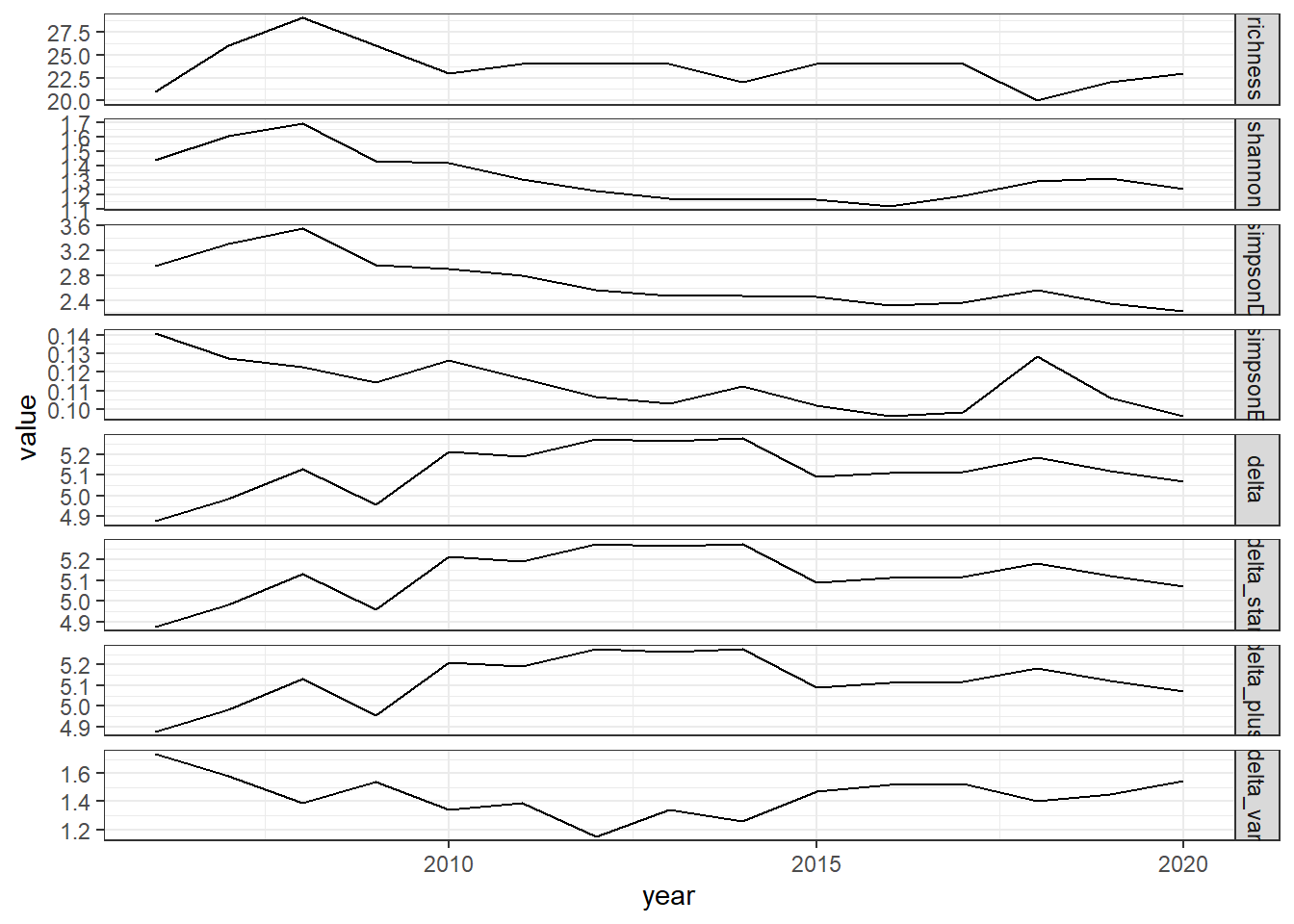
ggplot()+geom_line(data=all_melt_full2, aes(year,value))+facet_grid(rows = vars(variable), scales="free")+theme_bw()
grid.arrange(rich_full2, diversity_full2, evenness_full2,tax.distinct_full2, nrow=4)