Plots
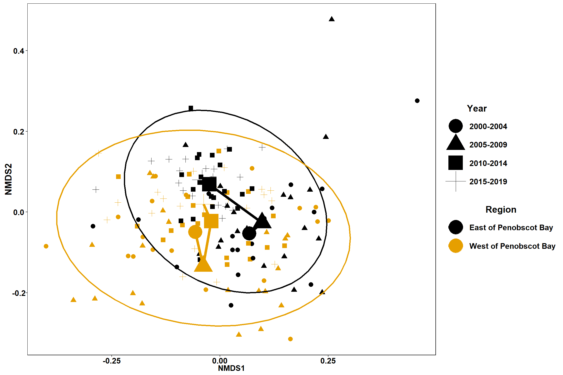
Region
#both seasons
data.scores_region<-filter(data.scores,Region_new!="Penobscot Bay")
#calculate center of ellipse for each region/year grouping
data.scores_2<-group_by(data.scores_region, Region_new, Year_groups)%>%
mutate(indicator=cur_group_id())
id<-dplyr::select(data.scores_2, Region_new, Year_groups, indicator)
id<-unique(id)
ctr<-NULL
Ncombo<-length(unique(data.scores_2$indicator))
for (i in 1:Ncombo) {
combos<- filter(data.scores_2, indicator==i)%>%
ungroup()%>%
dplyr::select(1:2)
ctr[[i]]<-MASS::cov.trob(combos)$center
}
d<-as.data.frame(ctr)
d<-as.data.frame(t(d))
d$indicator<-seq(1:8)
rownames(d)<-NULL
centers<-full_join(d,id)
p <- ggplot() +
geom_point(data=data.scores_region, aes(x = NMDS1, y = NMDS2, shape=factor(Year_groups),color=factor(Region_new)),size = 3)+
#geom_mark_ellipse(data=data.scores_region,aes(x=NMDS1,y=NMDS2,color=factor(Region_new)), size=1, alpha=0.15)+
stat_ellipse(data=data.scores_region, aes(x=NMDS1, y=NMDS2, color=Region_new),level = 0.95,size=1)+
scale_color_colorblind()+
# geom_text_repel(data= data.scores_region, aes(x= NMDS1, y=NMDS2, label= Year))+
labs(x = "NMDS1", colour = "Region", y = "NMDS2", shape = "Year")+
geom_point(data=centers, aes(NMDS1, NMDS2,shape=Year_groups, color=Region_new), size=10)+
geom_path(data=centers, aes(NMDS1, NMDS2, color=Region_new), size=2)
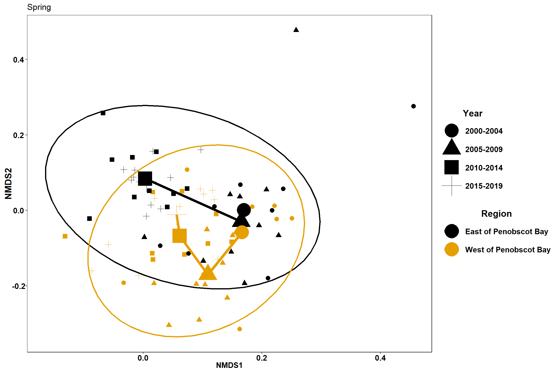
#spring
data.scores_region<-filter(data.scores,Region_new!="Penobscot Bay")%>%
filter(Season=="Spring")
#calculate center of ellipse for each region/year grouping
data.scores_2<-group_by(data.scores_region, Region_new, Year_groups, Season)%>%
mutate(indicator=cur_group_id())
id<-dplyr::select(data.scores_2, Region_new, Year_groups,Season, indicator)
id<-unique(id)
ctr<-NULL
Ncombo<-length(unique(data.scores_2$indicator))
for (i in 1:Ncombo) {
combos<- filter(data.scores_2, indicator==i)%>%
ungroup()%>%
dplyr::select(1:2)
ctr[[i]]<-MASS::cov.trob(combos)$center
}
d<-as.data.frame(ctr)
d<-as.data.frame(t(d))
d$indicator<-seq(1:8)
rownames(d)<-NULL
centers<-full_join(d,id)
p1 <- ggplot() +
geom_point(data=data.scores_region, aes(x = NMDS1, y = NMDS2, shape=factor(Year_groups),color=factor(Region_new)),size = 3)+
#geom_mark_ellipse(data=data.scores_region,aes(x=NMDS1,y=NMDS2,color=factor(Region_new)), size=1, alpha=0.15)+
stat_ellipse(data=data.scores_region, aes(x=NMDS1, y=NMDS2, color=Region_new),level = 0.95,size=1)+
scale_color_colorblind()+
# geom_text_repel(data= data.scores_region, aes(x= NMDS1, y=NMDS2, label= Year))+
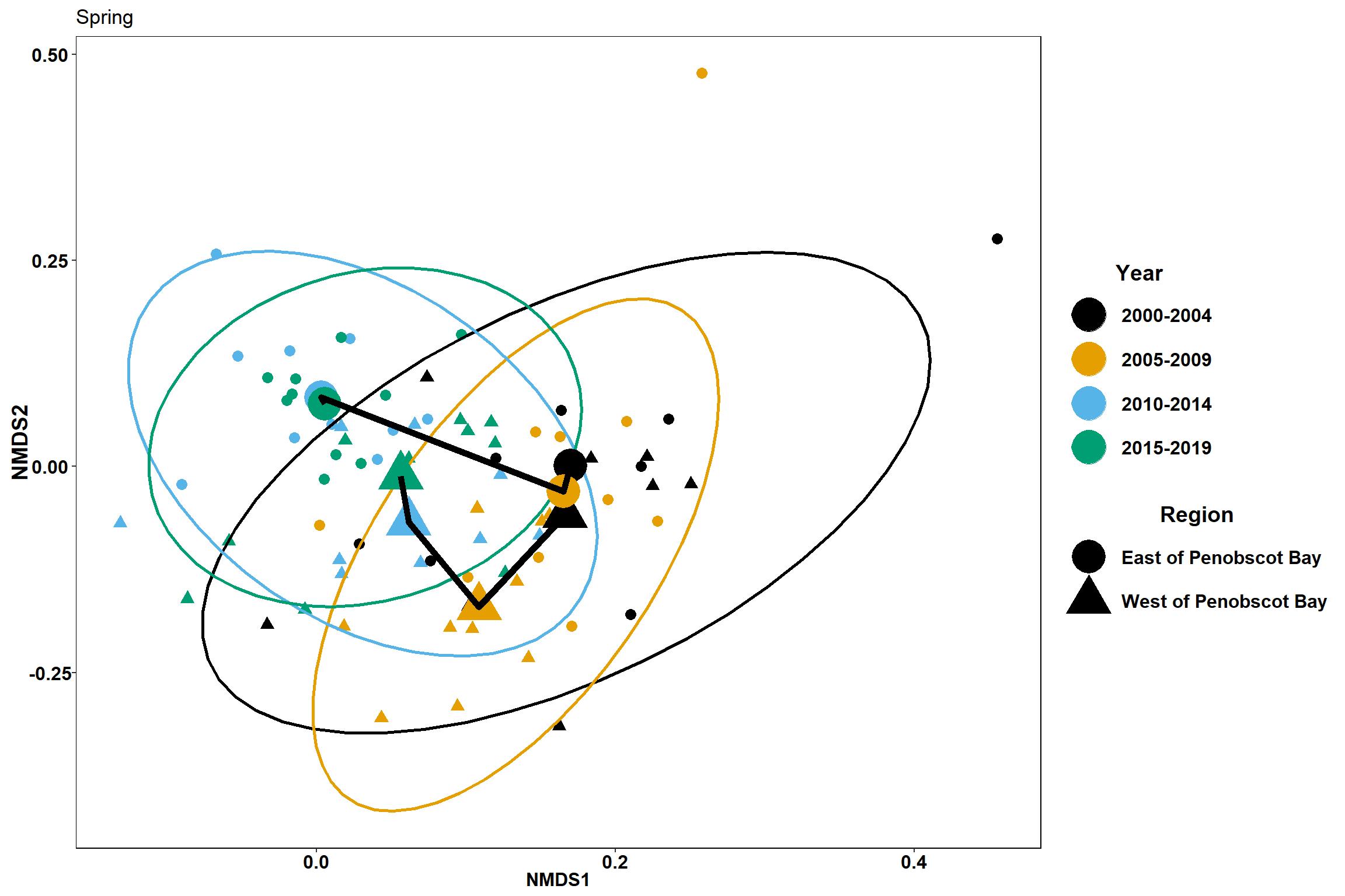
labs(x = "NMDS1", colour = "Region", y = "NMDS2", shape = "Year", title="Spring")+
geom_point(data=centers, aes(NMDS1, NMDS2,shape=Year_groups, color=Region_new), size=10)+
geom_path(data=centers, aes(NMDS1, NMDS2, color=Region_new), size=2)
#Fall
data.scores_region<-filter(data.scores,Region_new!="Penobscot Bay")%>%
filter(Season=="Fall")
#calculate center of ellipse for each region/year grouping
data.scores_2<-group_by(data.scores_region, Region_new, Year_groups, Season)%>%
mutate(indicator=cur_group_id())
id<-dplyr::select(data.scores_2, Region_new, Year_groups,Season, indicator)
id<-unique(id)
ctr<-NULL
Ncombo<-length(unique(data.scores_2$indicator))
for (i in 1:Ncombo) {
combos<- filter(data.scores_2, indicator==i)%>%
ungroup()%>%
dplyr::select(1:2)
ctr[[i]]<-MASS::cov.trob(combos)$center
}
d<-as.data.frame(ctr)
d<-as.data.frame(t(d))
d$indicator<-seq(1:8)
rownames(d)<-NULL
centers<-full_join(d,id)
p2 <- ggplot() +
geom_point(data=data.scores_region, aes(x = NMDS1, y = NMDS2, shape=factor(Year_groups),color=factor(Region_new)),size = 3)+
#geom_mark_ellipse(data=data.scores_region,aes(x=NMDS1,y=NMDS2,color=factor(Region_new)), size=1, alpha=0.15)+
stat_ellipse(data=data.scores_region, aes(x=NMDS1, y=NMDS2, color=Region_new),level = 0.95,size=1)+
scale_color_colorblind()+
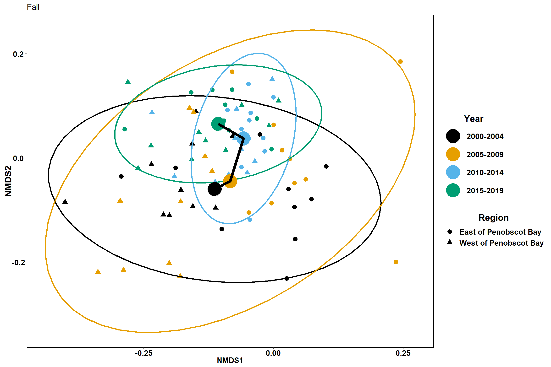
labs(x = "NMDS1", colour = "Region", y = "NMDS2", shape = "Year",title="Fall")+
geom_point(data=centers, aes(NMDS1, NMDS2, shape=Year_groups, color=Region_new), size=10)+
geom_path(data=centers, aes(NMDS1, NMDS2, color=Region_new), size=2)
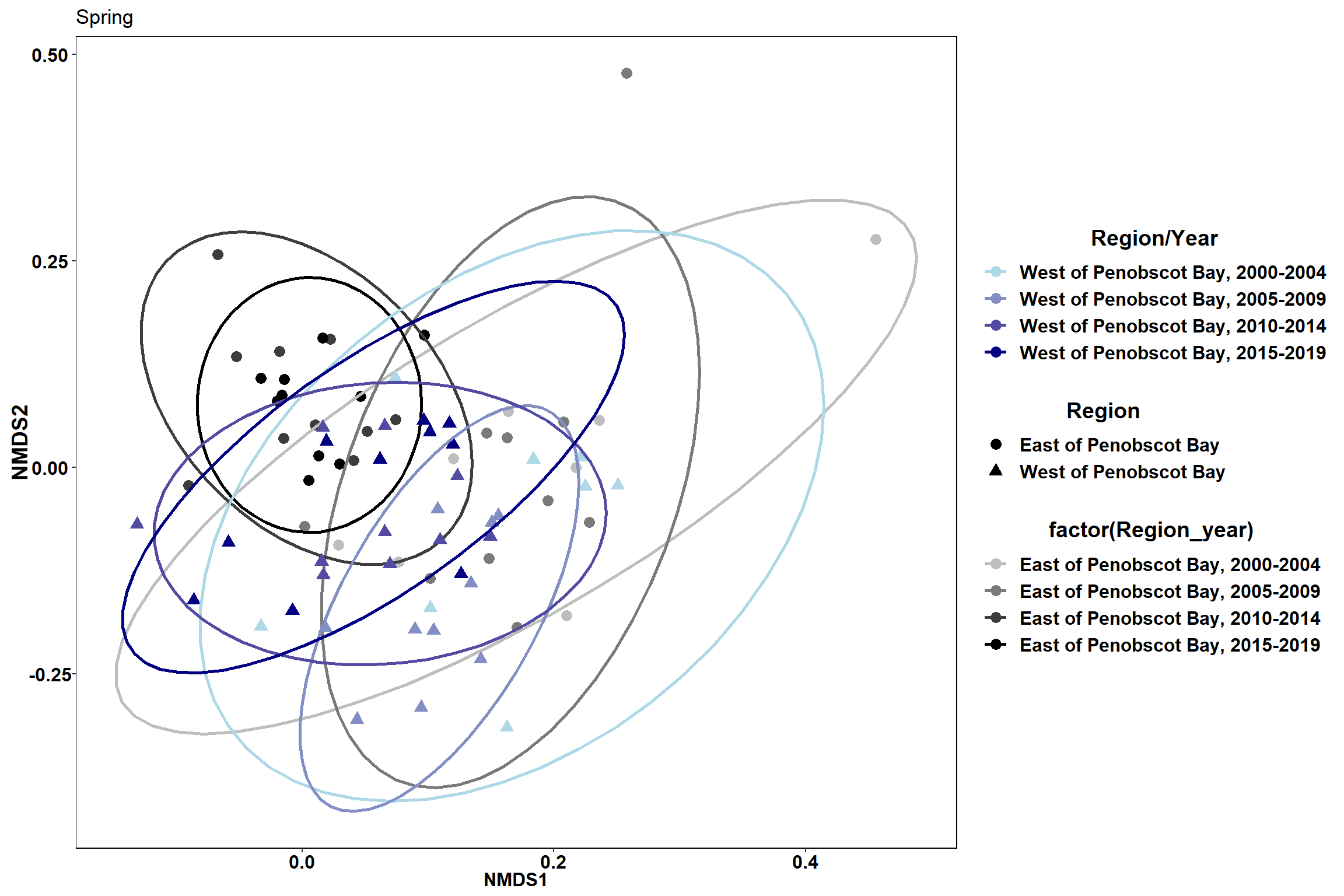
#Spring
data.scores_east<-filter(data.scores, Region_new=="East of Penobscot Bay")%>%
filter(Season=="Spring")
data.scores_west<-filter(data.scores, Region_new=="West of Penobscot Bay")%>%
filter(Season=="Spring")
p3<- ggplot() +
geom_point(data=data.scores_east, aes(x = NMDS1, y = NMDS2,color=factor(Region_year), shape=factor(Region_new)),size = 3)+
#geom_mark_ellipse(data=data.scores_east,aes(x=NMDS1,y=NMDS2,color=factor(Region_year)), size=1, alpha=0.15)+
stat_ellipse(data=data.scores_east, aes(x=NMDS1, y=NMDS2, color=Region_year),level = 0.95,size=1)+
scale_color_manual(values=scales::seq_gradient_pal("grey", "black", "Lab")(seq(0,1,length.out=4)))+
#geom_path(data=data.scores_east, aes(x=NMDS1,y=NMDS2,group=factor(Region_new)))+
#geom_text_repel(data=data.scores_east,aes(x=NMDS1,y=NMDS2,label=Year), size=4, fontface="bold", color="black")+
ggnewscale::new_scale_color()+
geom_point(data=data.scores_west, aes(x = NMDS1, y = NMDS2,color=factor(Region_year), shape=factor(Region_new)),size = 3)+
#geom_mark_ellipse(data=data.scores_west,aes(x=NMDS1,y=NMDS2,color=factor(Region_year)), size=1, alpha=0.15)+
stat_ellipse(data=data.scores_west, aes(x=NMDS1, y=NMDS2, color=Region_year),level = 0.95,size=1)+
scale_color_manual(values=scales::seq_gradient_pal("light blue", "navy", "Lab")(seq(0,1,length.out=4)))+
#geom_path(data=data.scores_west, aes(x=NMDS1,y=NMDS2,group=factor(Region_new)))+
#geom_text_repel(data=data.scores_west,aes(x=NMDS1,y=NMDS2,label=Year), size=4, fontface="bold", color="black")+
labs(x = "NMDS1", colour = "Region/Year", y = "NMDS2", shape = "Region", fill="Region/Year", title="Spring")
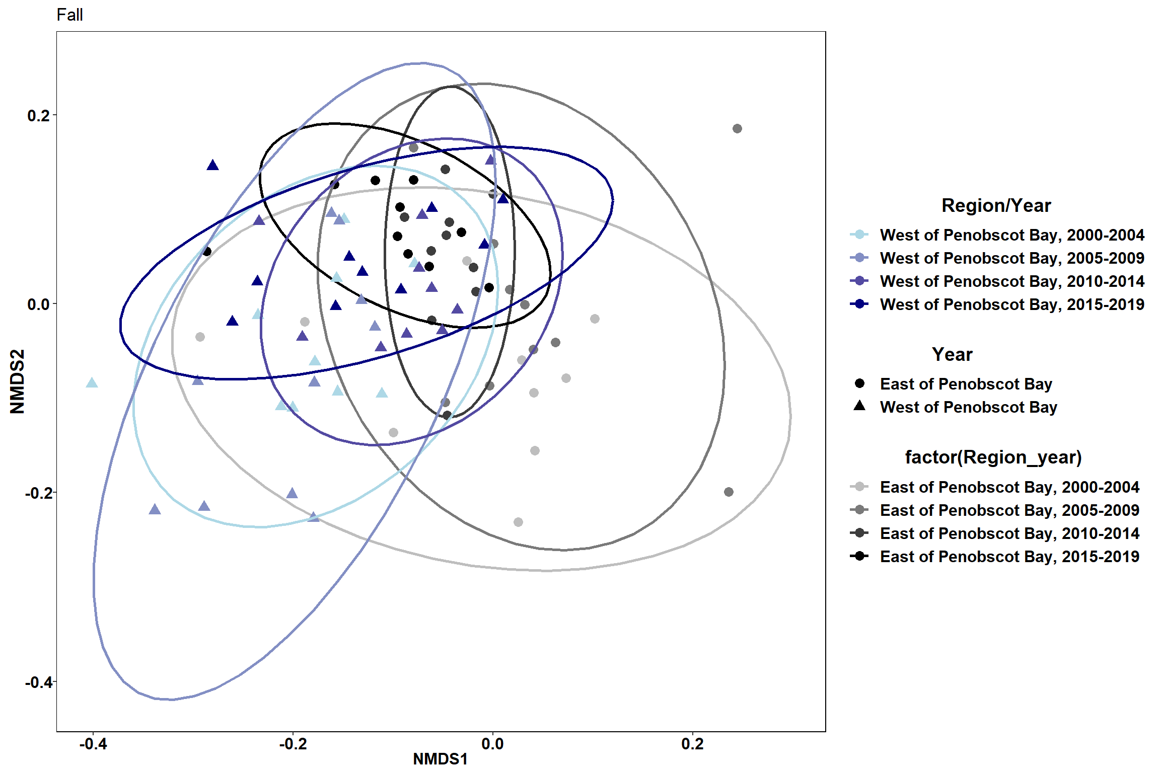
#Fall
data.scores_east<-filter(data.scores, Region_new=="East of Penobscot Bay")%>%
filter(Season=="Fall")
data.scores_west<-filter(data.scores, Region_new=="West of Penobscot Bay")%>%
filter(Season=="Fall")
p4<- ggplot() +
geom_point(data=data.scores_east, aes(x = NMDS1, y = NMDS2,color=factor(Region_year), shape=factor(Region_new)),size = 3)+
#geom_mark_ellipse(data=data.scores_east,aes(x=NMDS1,y=NMDS2,color=factor(Region_year)), size=1, alpha=0.15)+
stat_ellipse(data=data.scores_east, aes(x=NMDS1, y=NMDS2, color=Region_year),level = 0.95,size=1)+
scale_color_manual(values=scales::seq_gradient_pal("grey", "black", "Lab")(seq(0,1,length.out=4)))+
#geom_path(data=data.scores_east, aes(x=NMDS1,y=NMDS2,group=factor(Region_new)))+
#geom_text_repel(data=data.scores_east,aes(x=NMDS1,y=NMDS2,label=Year), size=4, fontface="bold", color="black")+
ggnewscale::new_scale_color()+
geom_point(data=data.scores_west, aes(x = NMDS1, y = NMDS2,color=factor(Region_year), shape=factor(Region_new)),size = 3)+
#geom_mark_ellipse(data=data.scores_west,aes(x=NMDS1,y=NMDS2,color=factor(Region_year)), size=1, alpha=0.15)+
stat_ellipse(data=data.scores_west, aes(x=NMDS1, y=NMDS2, color=Region_year),level = 0.95,size=1)+
scale_color_manual(values=scales::seq_gradient_pal("light blue", "navy", "Lab")(seq(0,1,length.out=4)))+
#geom_path(data=data.scores_west, aes(x=NMDS1,y=NMDS2,group=factor(Region_new)))+
#geom_text_repel(data=data.scores_west,aes(x=NMDS1,y=NMDS2,label=Year), size=4, fontface="bold", color="black")+
labs(x = "NMDS1", colour = "Region/Year", y = "NMDS2", shape = "Year", fill="Region/Year", title="Fall")
p
p1
p2
p3
p4
Time
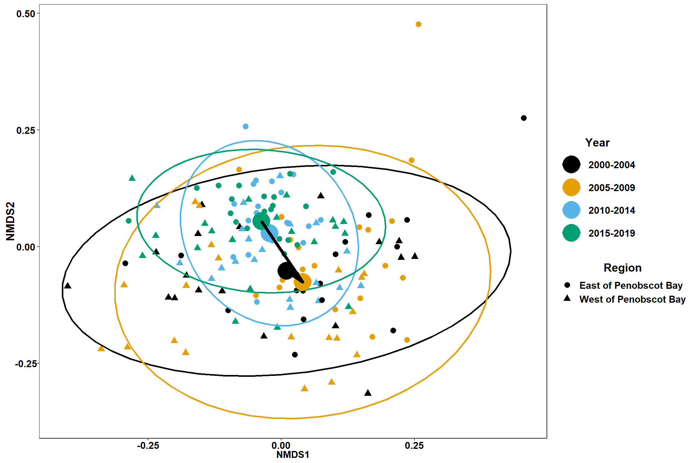
#both seasons
data.scores_region<-filter(data.scores,Region_new!="Penobscot Bay")
#centers for year plots
data.scores_2<-group_by(data.scores_region, Year_groups)%>%
mutate(indicator=cur_group_id())
id<-dplyr::select(data.scores_2, Year_groups, indicator)
id<-unique(id)
ctr<-NULL
Ncombo<-length(unique(data.scores_2$indicator))
for (i in 1:Ncombo) {
combos<- filter(data.scores_2, indicator==i)%>%
ungroup()%>%
dplyr::select(1:2)
ctr[[i]]<-MASS::cov.trob(combos)$center
}
d<-as.data.frame(ctr)
d<-as.data.frame(t(d))
d$indicator<-seq(1:4)
rownames(d)<-NULL
centers<-full_join(d,id)
p <- ggplot() +
geom_point(data=data.scores_region, aes(x = NMDS1, y = NMDS2,color=factor(Year_groups), shape=factor(Region_new)),size = 3)+
#geom_mark_ellipse(data=data.scores_region,aes(x=NMDS1,y=NMDS2,color=factor(Year_groups)), size=1, alpha=0.15)+
stat_ellipse(data=data.scores_region, aes(x=NMDS1, y=NMDS2, color=Year_groups),level = 0.95,size=1)+
scale_color_colorblind()+
labs(x = "NMDS1", colour = "Year", y = "NMDS2", shape = "Region")+
geom_point(data=centers, aes(NMDS1, NMDS2, color=Year_groups), size=10)+
geom_path(data=centers, aes(NMDS1, NMDS2), size=2)
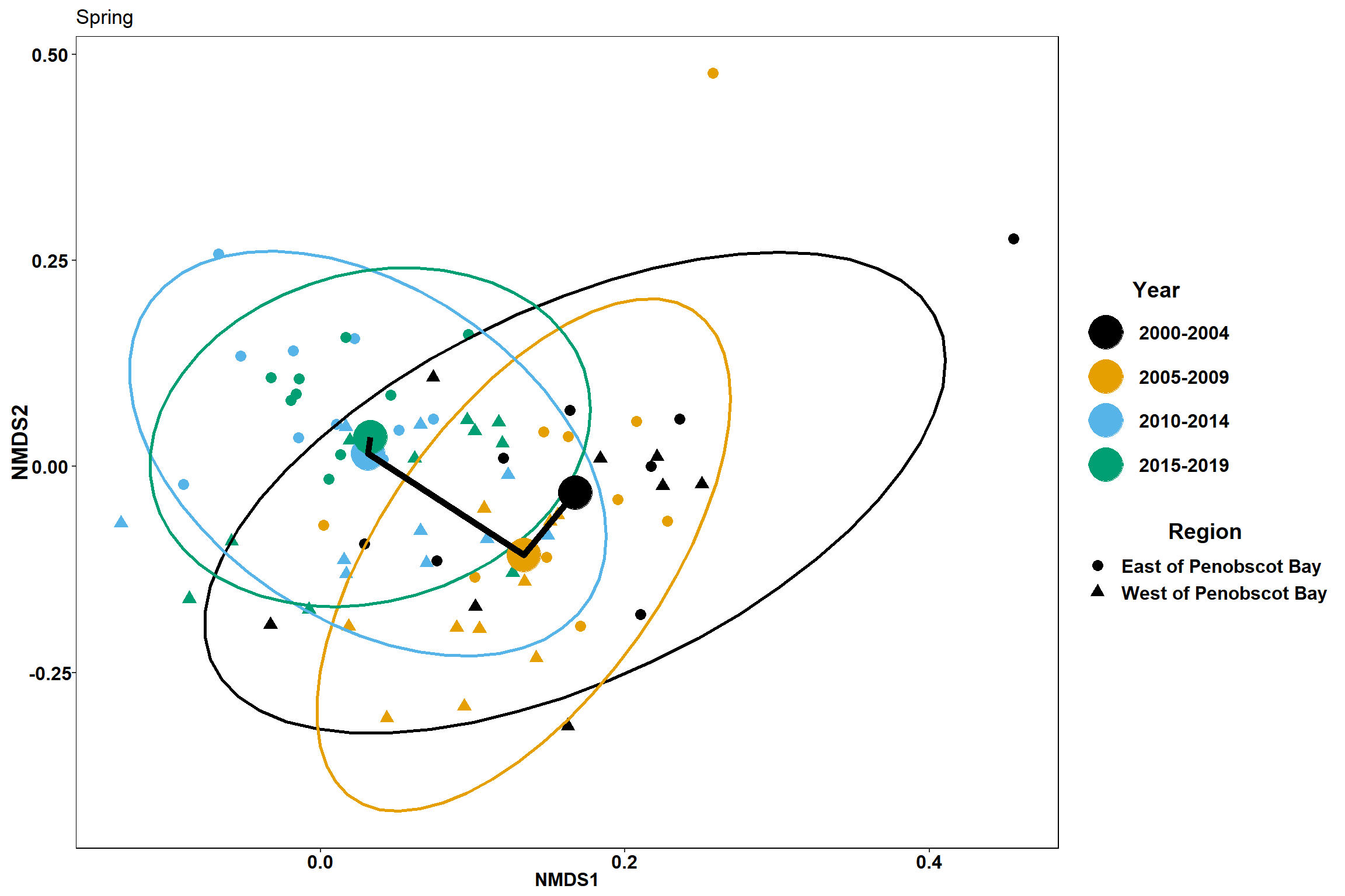
#Spring
data.scores_region<-filter(data.scores,Region_new!="Penobscot Bay")%>%
filter(Season=="Spring")
#centers for year plots
data.scores_2<-group_by(data.scores_region, Year_groups, Season)%>%
mutate(indicator=cur_group_id())
id<-dplyr::select(data.scores_2, Year_groups,Season, indicator)
id<-unique(id)
ctr<-NULL
Ncombo<-length(unique(data.scores_2$indicator))
for (i in 1:Ncombo) {
combos<- filter(data.scores_2, indicator==i)%>%
ungroup()%>%
dplyr::select(1:2)
ctr[[i]]<-MASS::cov.trob(combos)$center
}
d<-as.data.frame(ctr)
d<-as.data.frame(t(d))
d$indicator<-seq(1:4)
rownames(d)<-NULL
centers<-full_join(d,id)
p1 <- ggplot() +
geom_point(data=data.scores_region, aes(x = NMDS1, y = NMDS2,color=factor(Year_groups), shape=factor(Region_new)),size = 3)+
#geom_mark_ellipse(data=data.scores_region,aes(x=NMDS1,y=NMDS2,color=factor(Year_groups)), size=1, alpha=0.15)+
stat_ellipse(data=data.scores_region, aes(x=NMDS1, y=NMDS2, color=Year_groups),level = 0.95,size=1)+
scale_color_colorblind()+
labs(x = "NMDS1", colour = "Year", y = "NMDS2", shape = "Region", title="Spring")+
geom_point(data=centers, aes(NMDS1, NMDS2, color=Year_groups), size=10)+
geom_path(data=centers, aes(NMDS1, NMDS2), size=2)
#Fall
data.scores_region<-filter(data.scores,Region_new!="Penobscot Bay")%>%
filter(Season=="Fall")
#centers for year plots
data.scores_2<-group_by(data.scores_region, Year_groups, Season)%>%
mutate(indicator=cur_group_id())
id<-dplyr::select(data.scores_2, Year_groups,Season, indicator)
id<-unique(id)
ctr<-NULL
Ncombo<-length(unique(data.scores_2$indicator))
for (i in 1:Ncombo) {
combos<- filter(data.scores_2, indicator==i)%>%
ungroup()%>%
dplyr::select(1:2)
ctr[[i]]<-MASS::cov.trob(combos)$center
}
d<-as.data.frame(ctr)
d<-as.data.frame(t(d))
d$indicator<-seq(1:4)
rownames(d)<-NULL
centers<-full_join(d,id)
p2 <- ggplot() +
geom_point(data=data.scores_region, aes(x = NMDS1, y = NMDS2,color=factor(Year_groups), shape=factor(Region_new)),size = 3)+
#geom_mark_ellipse(data=data.scores_region,aes(x=NMDS1,y=NMDS2,color=factor(Year_groups)), size=1, alpha=0.15)+
stat_ellipse(data=data.scores_region, aes(x=NMDS1, y=NMDS2, color=Year_groups),level = 0.95,size=1)+
scale_color_colorblind()+
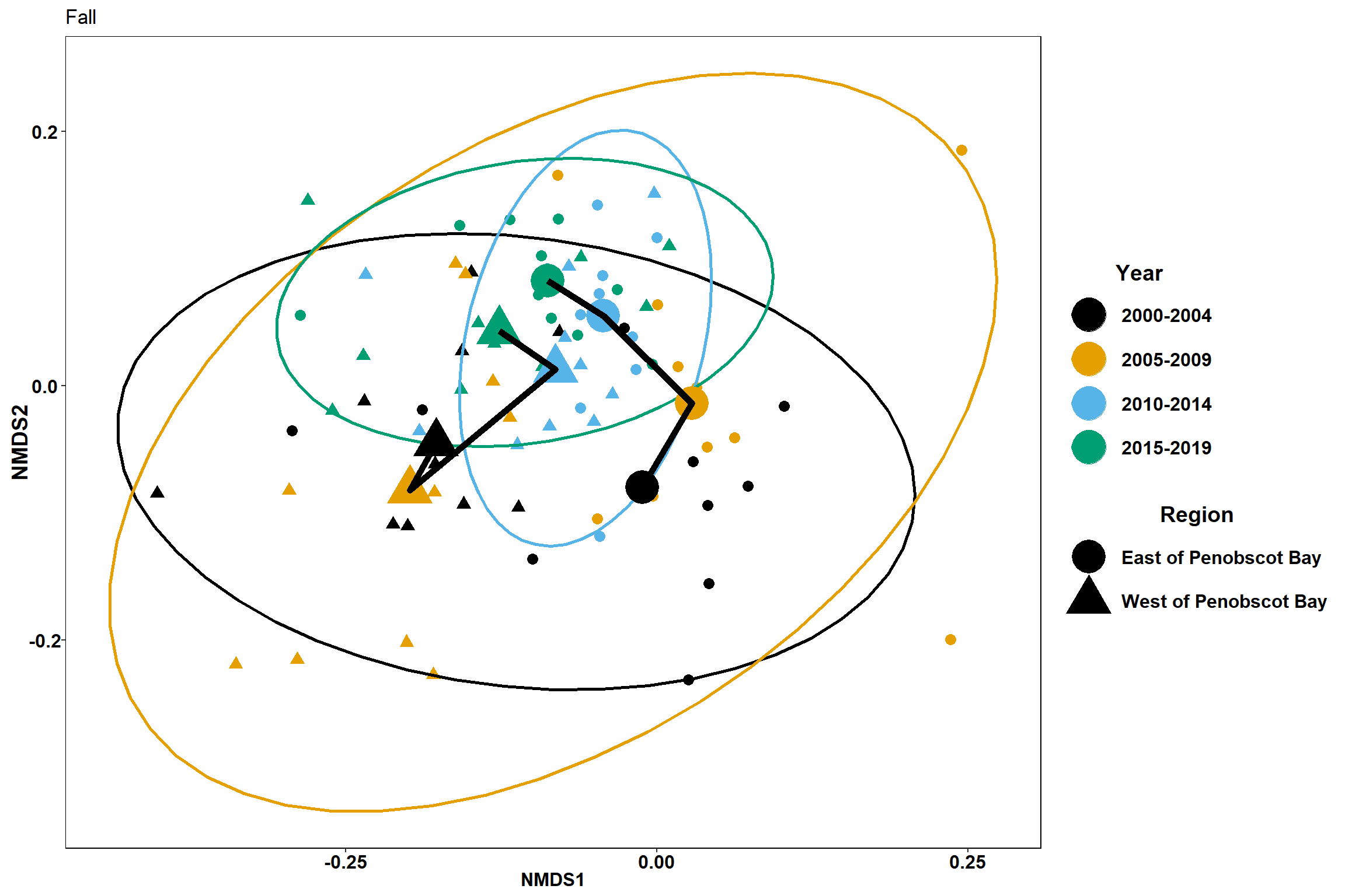
labs(x = "NMDS1", colour = "Year", y = "NMDS2", shape = "Region", title="Fall")+
geom_point(data=centers, aes(NMDS1, NMDS2, color=Year_groups), size=10)+
geom_path(data=centers, aes(NMDS1, NMDS2), size=2)
#Spring
data.scores_region<-filter(data.scores,Region_new!="Penobscot Bay")%>%
filter(Season=="Spring")
#centers for year plots
data.scores_2<-group_by(data.scores_region, Year_groups,Region_new, Season)%>%
mutate(indicator=cur_group_id())
id<-dplyr::select(data.scores_2, Year_groups,Season,Region_new, indicator)
id<-unique(id)
ctr<-NULL
Ncombo<-length(unique(data.scores_2$indicator))
for (i in 1:Ncombo) {
combos<- filter(data.scores_2, indicator==i)%>%
ungroup()%>%
dplyr::select(1:2)
ctr[[i]]<-MASS::cov.trob(combos)$center
}
d<-as.data.frame(ctr)
d<-as.data.frame(t(d))
d$indicator<-seq(1:8)
rownames(d)<-NULL
centers<-full_join(d,id)
p3 <- ggplot() +
geom_point(data=data.scores_region, aes(x = NMDS1, y = NMDS2,color=factor(Year_groups), shape=factor(Region_new)),size = 3)+
#geom_mark_ellipse(data=data.scores_region,aes(x=NMDS1,y=NMDS2,color=factor(Year_groups)), size=1, alpha=0.15)+
stat_ellipse(data=data.scores_region, aes(x=NMDS1, y=NMDS2, color=Year_groups),level = 0.95,size=1)+
scale_color_colorblind()+
labs(x = "NMDS1", colour = "Year", y = "NMDS2", shape = "Region", title="Spring")+
geom_point(data=centers, aes(NMDS1, NMDS2, color=Year_groups, shape=Region_new), size=10)+
geom_path(data=centers, aes(NMDS1, NMDS2, group=Region_new), size=2)
#Fall
data.scores_region<-filter(data.scores,Region_new!="Penobscot Bay")%>%
filter(Season=="Fall")
#centers for year plots
data.scores_2<-group_by(data.scores_region, Year_groups,Region_new, Season)%>%
mutate(indicator=cur_group_id())
id<-dplyr::select(data.scores_2, Year_groups,Season,Region_new, indicator)
id<-unique(id)
ctr<-NULL
Ncombo<-length(unique(data.scores_2$indicator))
for (i in 1:Ncombo) {
combos<- filter(data.scores_2, indicator==i)%>%
ungroup()%>%
dplyr::select(1:2)
ctr[[i]]<-MASS::cov.trob(combos)$center
}
d<-as.data.frame(ctr)
d<-as.data.frame(t(d))
d$indicator<-seq(1:8)
rownames(d)<-NULL
centers<-full_join(d,id)
p4 <- ggplot() +
geom_point(data=data.scores_region, aes(x = NMDS1, y = NMDS2,color=factor(Year_groups), shape=factor(Region_new)),size = 3)+
#geom_mark_ellipse(data=data.scores_region,aes(x=NMDS1,y=NMDS2,color=factor(Year_groups)), size=1, alpha=0.15)+
stat_ellipse(data=data.scores_region, aes(x=NMDS1, y=NMDS2, color=Year_groups),level = 0.95,size=1)+
scale_color_colorblind()+
labs(x = "NMDS1", colour = "Year", y = "NMDS2", shape = "Region", title="Fall")+
geom_point(data=centers, aes(NMDS1, NMDS2, color=Year_groups, shape=Region_new), size=10)+
geom_path(data=centers, aes(NMDS1, NMDS2, group=Region_new), size=2)
p
p1
p2
p3
p4
Season
#all regions
#centers for year plots
data.scores_2<-group_by(data.scores, Year_groups, Season)%>%
mutate(indicator=cur_group_id())
id<-dplyr::select(data.scores_2, Year_groups,Season, indicator)
id<-unique(id)
ctr<-NULL
Ncombo<-length(unique(data.scores_2$indicator))
for (i in 1:Ncombo) {
combos<- filter(data.scores_2, indicator==i)%>%
ungroup()%>%
dplyr::select(1:2)
ctr[[i]]<-MASS::cov.trob(combos)$center
}
d<-as.data.frame(ctr)
d<-as.data.frame(t(d))
d$indicator<-seq(1:8)
rownames(d)<-NULL
centers<-full_join(d,id)
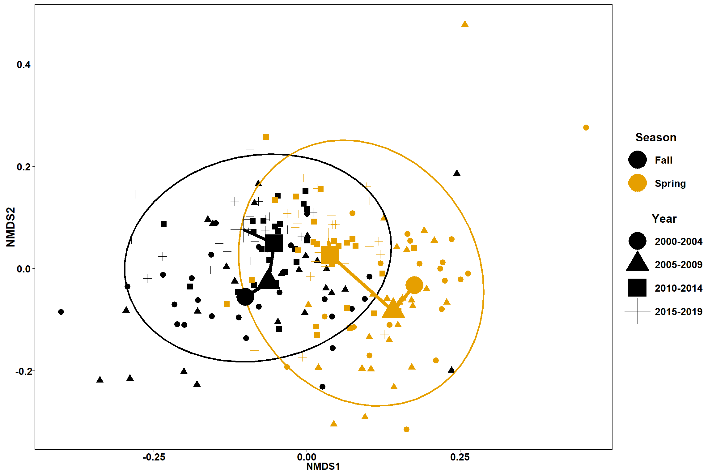
p <- ggplot(data.scores, aes(x = NMDS1, y = NMDS2)) +
geom_point(size = 3, aes(shape=factor(Year_groups), color=factor(Season)))+
stat_ellipse(data=data.scores, aes(x=NMDS1, y=NMDS2, color=Season),level = 0.95,size=1)+
#geom_mark_ellipse(aes(color=factor(Season)), size=1, alpha=0.15)+
scale_color_colorblind()+
labs(x = "NMDS1", colour = "Season", y = "NMDS2", shape = "Year", fill="Season")+
geom_point(data=centers, aes(NMDS1, NMDS2, color=Season, shape=Year_groups), size=10)+
geom_path(data=centers, aes(NMDS1, NMDS2, color=Season), size=2)
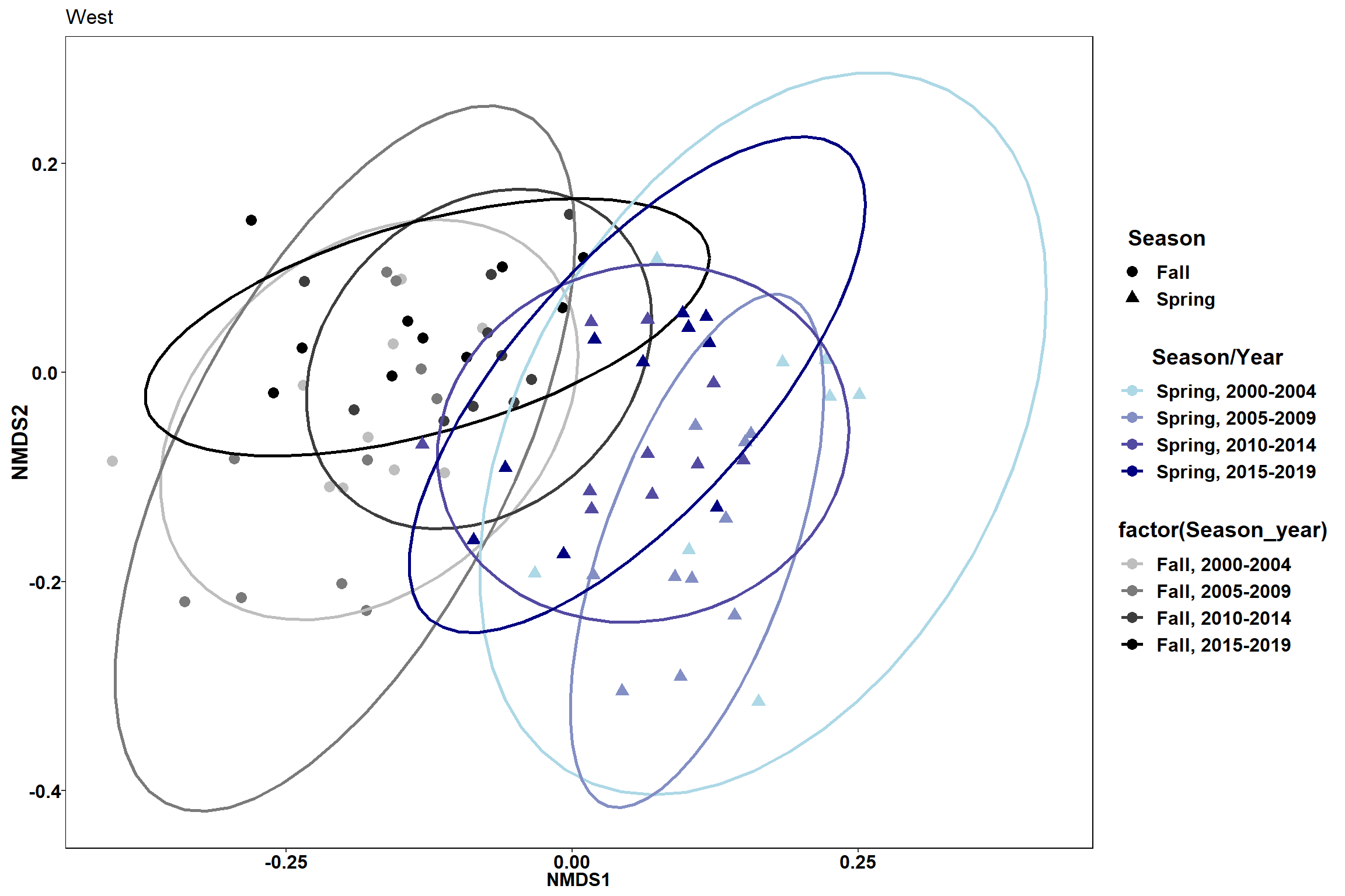
#ellipse season and year plot
data.scores_west<-filter(data.scores, Region_new=="West of Penobscot Bay")
#centers for year plots
data.scores_2<-group_by(data.scores_west, Year_groups,Region_new, Season)%>%
mutate(indicator=cur_group_id())
id<-dplyr::select(data.scores_2, Year_groups,Season,Region_new, indicator)
id<-unique(id)
ctr<-NULL
Ncombo<-length(unique(data.scores_2$indicator))
for (i in 1:Ncombo) {
combos<- filter(data.scores_2, indicator==i)%>%
ungroup()%>%
dplyr::select(1:2)
ctr[[i]]<-MASS::cov.trob(combos)$center
}
d<-as.data.frame(ctr)
d<-as.data.frame(t(d))
d$indicator<-seq(1:8)
rownames(d)<-NULL
centers<-full_join(d,id)
#West
p1 <- ggplot(data.scores_west, aes(x = NMDS1, y = NMDS2)) +
geom_point(size = 3, aes(shape=factor(Year_groups), color=factor(Season)))+
stat_ellipse(data=data.scores_west, aes(x=NMDS1, y=NMDS2, color=Season),level = 0.95,size=1)+
#geom_mark_ellipse(aes(color=factor(Season)), size=1, alpha=0.15)+
scale_color_colorblind()+
labs(x = "NMDS1", colour = "Season", y = "NMDS2", shape = "Year", fill="Season", title="West")+
geom_point(data=centers, aes(NMDS1, NMDS2, color=Season, shape=Year_groups), size=10)+
geom_path(data=centers, aes(NMDS1, NMDS2, color=Season), size=2)
#East
data.scores_east<-filter(data.scores, Region_new=="East of Penobscot Bay")
#centers for year plots
data.scores_2<-group_by(data.scores_east, Year_groups,Region_new, Season)%>%
mutate(indicator=cur_group_id())
id<-dplyr::select(data.scores_2, Year_groups,Season,Region_new, indicator)
id<-unique(id)
ctr<-NULL
Ncombo<-length(unique(data.scores_2$indicator))
for (i in 1:Ncombo) {
combos<- filter(data.scores_2, indicator==i)%>%
ungroup()%>%
dplyr::select(1:2)
ctr[[i]]<-MASS::cov.trob(combos)$center
}
d<-as.data.frame(ctr)
d<-as.data.frame(t(d))
d$indicator<-seq(1:8)
rownames(d)<-NULL
centers<-full_join(d,id)
p2 <- ggplot(data.scores_east, aes(x = NMDS1, y = NMDS2)) +
geom_point(size = 3, aes(shape=factor(Year_groups), color=factor(Season)))+
stat_ellipse(data=data.scores_east, aes(x=NMDS1, y=NMDS2, color=Season),level = 0.95,size=1)+
#geom_mark_ellipse(aes(color=factor(Season)), size=1, alpha=0.15)+
scale_color_colorblind()+
labs(x = "NMDS1", colour = "Season", y = "NMDS2", shape = "Year", fill="Season", title="East")+
geom_point(data=centers, aes(NMDS1, NMDS2, color=Season, shape=Year_groups), size=10)+
geom_path(data=centers, aes(NMDS1, NMDS2, color=Season), size=2)
#West
data.scores_spring<-filter(data.scores, Season=="Spring")%>%
filter(Region_new=="West of Penobscot Bay")
data.scores_fall<-filter(data.scores, Season=="Fall")%>%
filter(Region_new=="West of Penobscot Bay")
p3 <- ggplot() +
geom_point(data=data.scores_fall, aes(x = NMDS1, y = NMDS2,color=factor(Season_year), shape=factor(Season)),size = 3)+
#geom_mark_ellipse(data=data.scores_fall,aes(x=NMDS1,y=NMDS2,color=factor(Season_year)), size=1, alpha=0.15)+
stat_ellipse(data=data.scores_fall, aes(x=NMDS1, y=NMDS2, color=Season_year),level = 0.95,size=1)+
scale_color_manual(values=scales::seq_gradient_pal("grey", "black", "Lab")(seq(0,1,length.out=4)))+
#geom_path(data=data.scores_fall, aes(x=NMDS1,y=NMDS2,group=factor(Season)))+
#geom_text_repel(data=data.scores_fall,aes(x=NMDS1,y=NMDS2,label=Year), size=4, fontface="bold", color="black")+
ggnewscale::new_scale_color()+
geom_point(data=data.scores_spring, aes(x = NMDS1, y = NMDS2,color=factor(Season_year), shape=factor(Season)),size = 3)+
#geom_mark_ellipse(data=data.scores_spring,aes(x=NMDS1,y=NMDS2,color=factor(Season_year)), size=1, alpha=0.15)+
stat_ellipse(data=data.scores_spring, aes(x=NMDS1, y=NMDS2, color=Season_year),level = 0.95,size=1)+
scale_color_manual(values=scales::seq_gradient_pal("light blue", "navy", "Lab")(seq(0,1,length.out=4)))+
#geom_path(data=data.scores_spring, aes(x=NMDS1,y=NMDS2,group=factor(Season)),color="navy")+
#geom_text_repel(data=data.scores_spring,aes(x=NMDS1,y=NMDS2,label=Year), size=4, fontface="bold", color="black")+
labs(x = "NMDS1", colour = "Season/Year", y = "NMDS2", shape = "Season", fill="Season/Year", title="West")
#East
data.scores_spring<-filter(data.scores, Season=="Spring")%>%
filter(Region_new=="East of Penobscot Bay")
data.scores_fall<-filter(data.scores, Season=="Fall")%>%
filter(Region_new=="East of Penobscot Bay")
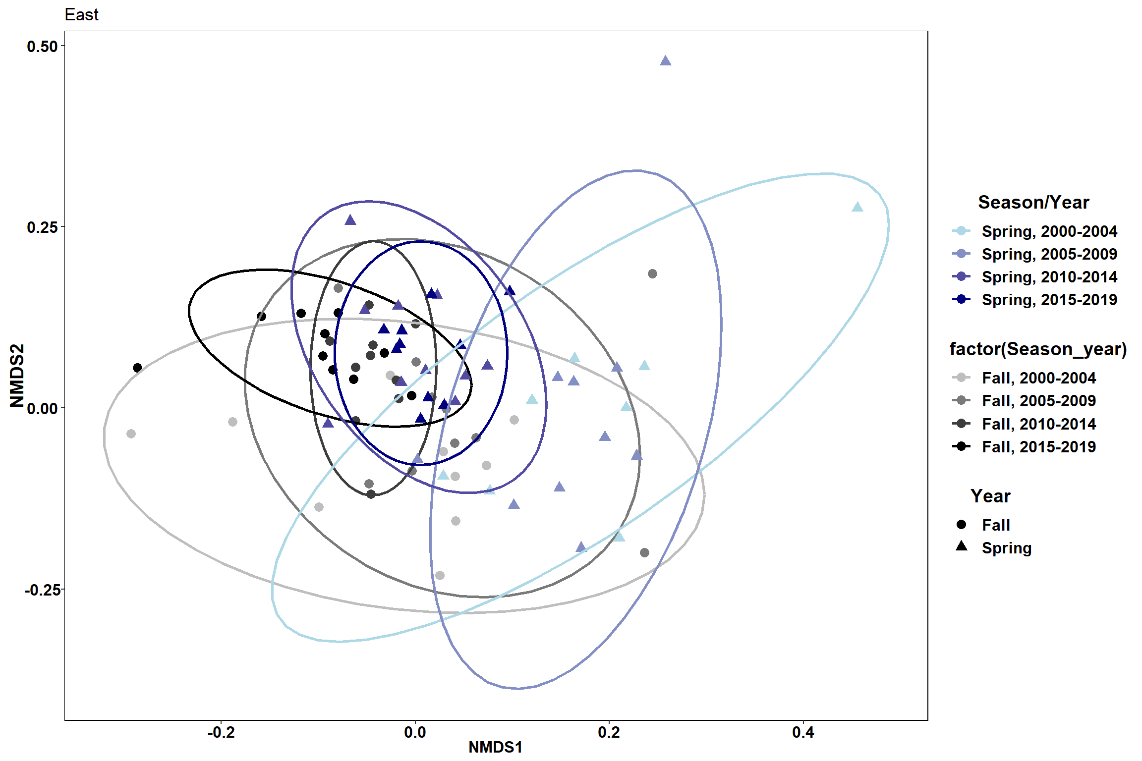
p4 <- ggplot() +
geom_point(data=data.scores_fall, aes(x = NMDS1, y = NMDS2,color=factor(Season_year), shape=factor(Season)),size = 3)+
#geom_mark_ellipse(data=data.scores_fall,aes(x=NMDS1,y=NMDS2,color=factor(Season_year)), size=1, alpha=0.15)+
stat_ellipse(data=data.scores_fall, aes(x=NMDS1, y=NMDS2, color=Season_year),level = 0.95,size=1)+
scale_color_manual(values=scales::seq_gradient_pal("grey", "black", "Lab")(seq(0,1,length.out=4)))+
#geom_path(data=data.scores_fall, aes(x=NMDS1,y=NMDS2,group=factor(Season)))+
#geom_text_repel(data=data.scores_fall,aes(x=NMDS1,y=NMDS2,label=Year), size=4, fontface="bold", color="black")+
ggnewscale::new_scale_color()+
geom_point(data=data.scores_spring, aes(x = NMDS1, y = NMDS2,color=factor(Season_year), shape=factor(Season)),size = 3)+
#geom_mark_ellipse(data=data.scores_spring,aes(x=NMDS1,y=NMDS2,color=factor(Season_year)), size=1, alpha=0.15)+
stat_ellipse(data=data.scores_spring, aes(x=NMDS1, y=NMDS2, color=Season_year),level = 0.95,size=1)+
scale_color_manual(values=scales::seq_gradient_pal("light blue", "navy", "Lab")(seq(0,1,length.out=4)))+
#geom_path(data=data.scores_spring, aes(x=NMDS1,y=NMDS2,group=factor(Season)),color="navy")+
#geom_text_repel(data=data.scores_spring,aes(x=NMDS1,y=NMDS2,label=Year), size=4, fontface="bold", color="black")+
labs(x = "NMDS1", colour = "Season/Year", y = "NMDS2", shape = "Year", fill="Season/Year", title="East")
p
p1
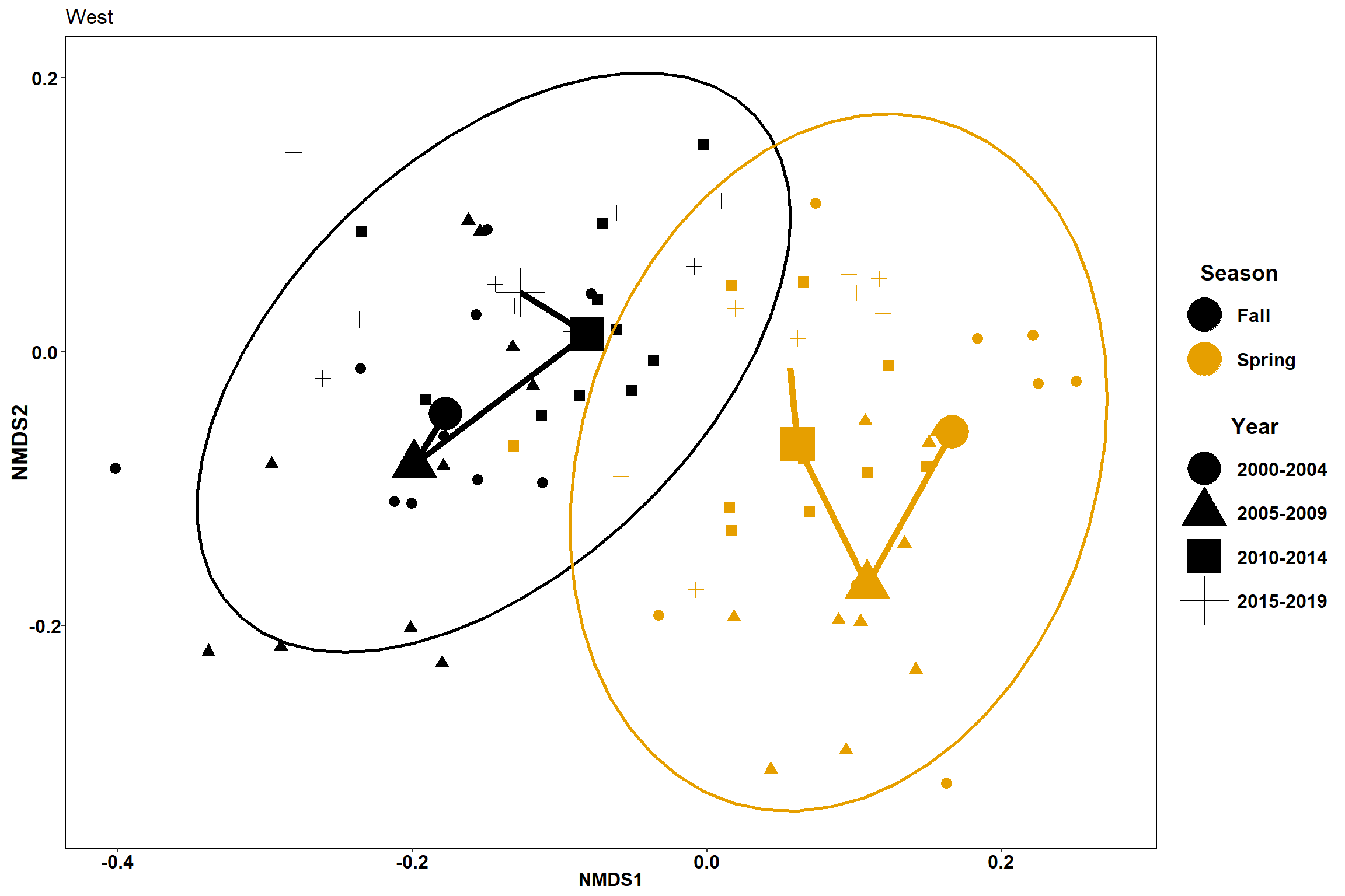
p2
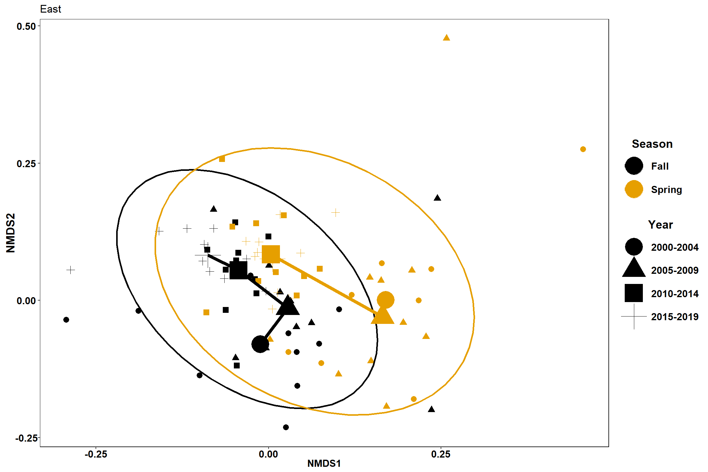
p3
p4