Analysis of Similarity and Analysis of Variance
Data- Biomass of top 50 species
- average across depth strata using the NOAA IEA technical document
- calculate dissimilarity matrix with Bray-Curtis distances
#load libraries
library(tidyverse)
library(vegan)
library(pairwiseAdonis)
library(indicspecies)
library(here)
library(rmarkdown)
library(gridExtra)

#bring in species matrix for analysis
trawl_data_arrange<-read.csv(here("Data/species_biomass_matrix.csv"))[-1]

#separate meta data from matrix
ME_group_data<-trawl_data_arrange[, c(1,2,3,54,55,56,57,58)]
ME_NMDS_data<-as.matrix(trawl_data_arrange[,4:53])

#calculate dissimilarity matrix for tests
trawl_dist<-vegdist(ME_NMDS_data,distance="bray")

paged_table(head(trawl_data_arrange))
Analysis of similarity (Anosim)
- tests statistically whether there is a significant difference between two or more groups
- works by testing if distances between groups are greater than within groups
- significant values mean that there is a statistically significant difference in the communities between the groups
- R statistic closer to 1 is more dissimilar
Region
#region
ano_region<- anosim(trawl_dist, trawl_data_arrange$Region, permutations = 999)
ano_region #regions are statistically different communities
##
## Call:
## anosim(x = trawl_dist, grouping = trawl_data_arrange$Region, permutations = 999)
## Dissimilarity: bray
##
## ANOSIM statistic R: 0.2409
## Significance: 0.001
##
## Permutation: free
## Number of permutations: 999summary(ano_region)##
## Call:
## anosim(x = trawl_dist, grouping = trawl_data_arrange$Region, permutations = 999)
## Dissimilarity: bray
##
## ANOSIM statistic R: 0.2409
## Significance: 0.001
##
## Permutation: free
## Number of permutations: 999
##
## Upper quantiles of permutations (null model):
## 90% 95% 97.5% 99%
## 0.0106 0.0142 0.0172 0.0206
##
## Dissimilarity ranks between and within classes:
## 0% 25% 50% 75% 100% N
## Between 4 5339.25 10126.5 14569.75 18915 15210
## 1 47 4152.00 8749.0 14402.00 18739 741
## 2 9 3263.00 7841.0 12723.00 18816 741
## 3 2 2364.00 6163.0 10546.00 18845 741
## 4 1 2319.00 6086.0 11106.00 18907 741
## 5 11 2575.00 5686.0 9835.00 18380 741plot(ano_region) #regions don't look very different in plot though...confidence bands all overlap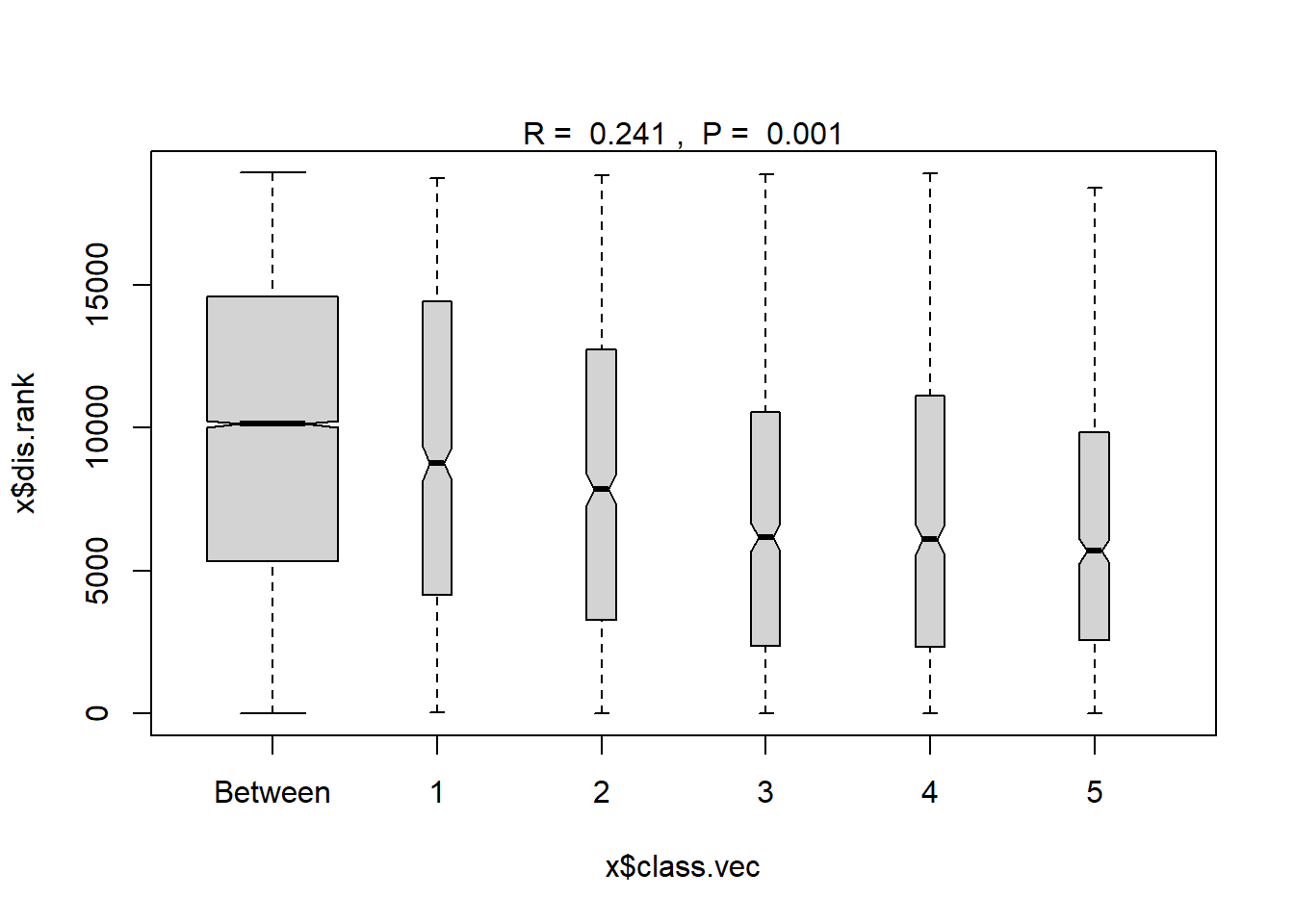
Region grouped
#region
ano_region_groups<- anosim(trawl_dist, trawl_data_arrange$REGION_NEW, permutations = 999)
ano_region_groups #regions are statistically different communities
##
## Call:
## anosim(x = trawl_dist, grouping = trawl_data_arrange$REGION_NEW, permutations = 999)
## Dissimilarity: bray
##
## ANOSIM statistic R: 0.1356
## Significance: 0.001
##
## Permutation: free
## Number of permutations: 999summary(ano_region_groups)##
## Call:
## anosim(x = trawl_dist, grouping = trawl_data_arrange$REGION_NEW, permutations = 999)
## Dissimilarity: bray
##
## ANOSIM statistic R: 0.1356
## Significance: 0.001
##
## Permutation: free
## Number of permutations: 999
##
## Upper quantiles of permutations (null model):
## 90% 95% 97.5% 99%
## 0.0194 0.0262 0.0322 0.0366
##
## Dissimilarity ranks between and within classes:
## 0% 25% 50% 75% 100% N
## Between 4 5348.0 10153.5 14585.5 18915 12168
## East of Penobscot Bay 1 3285.5 7245.0 12459.5 18907 3003
## Penobscot Bay 2 2364.0 6163.0 10546.0 18845 741
## West of Penobscot Bay 9 4921.0 9748.0 14430.0 18860 3003plot(ano_region_groups) #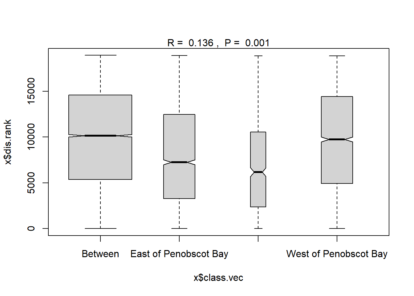
Year
#Time
ano_year<- anosim(trawl_dist, trawl_data_arrange$Year, permutations = 999)
ano_year #years are statistically different communities
##
## Call:
## anosim(x = trawl_dist, grouping = trawl_data_arrange$Year, permutations = 999)
## Dissimilarity: bray
##
## ANOSIM statistic R: 0.1252
## Significance: 0.001
##
## Permutation: free
## Number of permutations: 999summary(ano_year)##
## Call:
## anosim(x = trawl_dist, grouping = trawl_data_arrange$Year, permutations = 999)
## Dissimilarity: bray
##
## ANOSIM statistic R: 0.1252
## Significance: 0.001
##
## Permutation: free
## Number of permutations: 999
##
## Upper quantiles of permutations (null model):
## 90% 95% 97.5% 99%
## 0.0209 0.0273 0.0309 0.0363
##
## Dissimilarity ranks between and within classes:
## 0% 25% 50% 75% 100% N
## Between 1 4812.25 9534.5 14222.75 18915 18050
## 2000 217 4819.50 6612.5 9320.00 13344 10
## 2001 525 5418.00 12824.0 16868.00 18217 45
## 2002 619 6225.00 11209.0 13296.00 17389 45
## 2003 99 5655.00 10274.0 15244.00 18230 45
## 2004 260 9688.00 15280.0 17844.00 18887 45
## 2005 567 6315.00 10597.0 15396.00 18738 45
## 2006 198 6976.00 12562.0 15194.00 18221 45
## 2007 2131 9788.00 15651.0 17493.00 18900 45
## 2008 559 6095.00 11538.0 16202.00 18430 45
## 2009 266 5985.00 10139.0 12380.00 16642 45
## 2010 58 2203.00 6548.0 9759.00 14837 45
## 2011 457 4235.00 10369.0 13419.00 17082 45
## 2012 133 1364.00 3343.0 4590.00 10153 45
## 2013 18 795.00 2333.0 3796.00 11260 45
## 2014 6 1516.00 4963.0 9125.00 16084 45
## 2015 380 3017.00 5877.0 10700.00 17347 45
## 2016 70 1749.00 4757.0 7694.00 14871 45
## 2017 35 1168.00 4137.0 7191.00 14935 45
## 2018 12 3428.00 9051.0 13573.00 17500 45
## 2019 16 1930.00 4588.0 9241.00 16238 45plot(ano_year)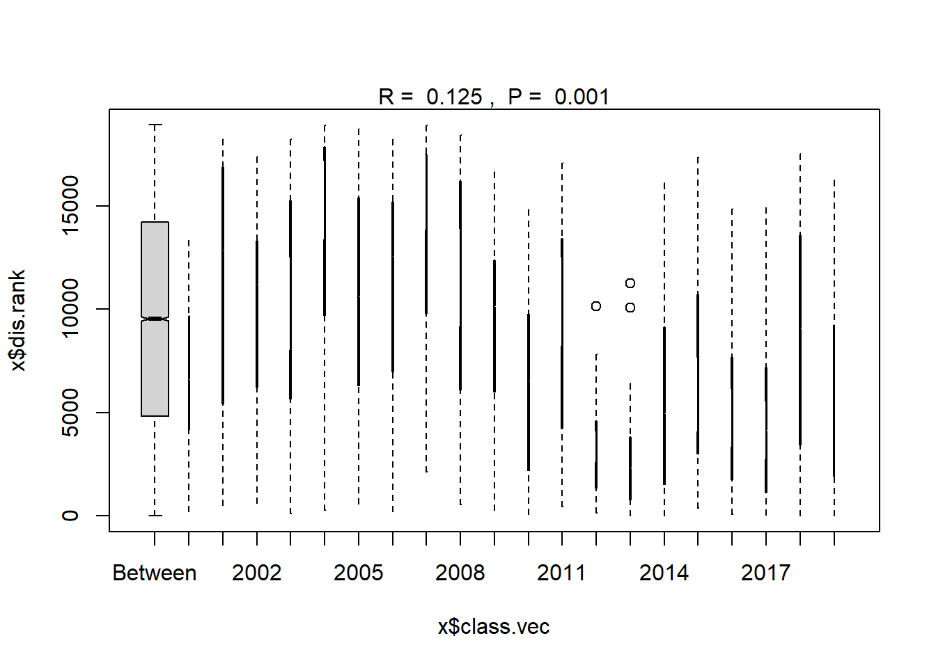
Year blocks
#Year blocks
ano_year_blocks<- anosim(trawl_dist, trawl_data_arrange$YEAR_GROUPS, permutations = 999)
ano_year_blocks #years are statistically different communities
##
## Call:
## anosim(x = trawl_dist, grouping = trawl_data_arrange$YEAR_GROUPS, permutations = 999)
## Dissimilarity: bray
##
## ANOSIM statistic R: 0.1698
## Significance: 0.001
##
## Permutation: free
## Number of permutations: 999summary(ano_year_blocks)##
## Call:
## anosim(x = trawl_dist, grouping = trawl_data_arrange$YEAR_GROUPS, permutations = 999)
## Dissimilarity: bray
##
## ANOSIM statistic R: 0.1698
## Significance: 0.001
##
## Permutation: free
## Number of permutations: 999
##
## Upper quantiles of permutations (null model):
## 90% 95% 97.5% 99%
## 0.0102 0.0133 0.0162 0.0195
##
## Dissimilarity ranks between and within classes:
## 0% 25% 50% 75% 100% N
## Between 1 5308.25 9966 14517.50 18915 14250
## 2000-2004 54 5768.50 11052 15452.75 18913 990
## 2005-2009 15 6208.00 11413 15720.00 18909 1225
## 2010-2014 6 2086.00 4807 8907.00 17501 1225
## 2015-2019 3 2053.00 5370 10302.00 18480 1225plot(ano_year_blocks)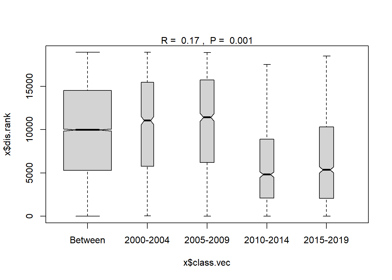
Analysis of variance (Adonis)
- Permanova
- tests whether there is a difference between means of groups
- works by calculating the sum of squares from the centroid of the group
Region
adonis<-adonis2(trawl_dist~Region, data=ME_group_data, by="terms", permutations = 9999)
adonis
## Permutation test for adonis under reduced model
## Terms added sequentially (first to last)
## Permutation: free
## Number of permutations: 9999
##
## adonis2(formula = trawl_dist ~ Region, data = ME_group_data, permutations = 9999, by = "terms")
## Df SumOfSqs R2 F Pr(>F)
## Region 1 2.4733 0.08292 17.451 1e-04 ***
## Residual 193 27.3532 0.91708
## Total 194 29.8265 1.00000
## ---
## Signif. codes: 0 '***' 0.001 '**' 0.01 '*' 0.05 '.' 0.1 ' ' 1summary(adonis)## Df SumOfSqs R2 F
## Min. : 1.0 Min. : 2.473 Min. :0.08292 Min. :17.45
## 1st Qu.: 97.0 1st Qu.:14.913 1st Qu.:0.50000 1st Qu.:17.45
## Median :193.0 Median :27.353 Median :0.91708 Median :17.45
## Mean :129.3 Mean :19.884 Mean :0.66667 Mean :17.45
## 3rd Qu.:193.5 3rd Qu.:28.590 3rd Qu.:0.95854 3rd Qu.:17.45
## Max. :194.0 Max. :29.826 Max. :1.00000 Max. :17.45
## NA's :2
## Pr(>F)
## Min. :1e-04
## 1st Qu.:1e-04
## Median :1e-04
## Mean :1e-04
## 3rd Qu.:1e-04
## Max. :1e-04
## NA's :2Year
adonis<-adonis2(trawl_dist~Year, data=ME_group_data, by="terms", permutations = 9999)
adonis
## Permutation test for adonis under reduced model
## Terms added sequentially (first to last)
## Permutation: free
## Number of permutations: 9999
##
## adonis2(formula = trawl_dist ~ Year, data = ME_group_data, permutations = 9999, by = "terms")
## Df SumOfSqs R2 F Pr(>F)
## Year 1 2.3702 0.07947 16.661 1e-04 ***
## Residual 193 27.4563 0.92053
## Total 194 29.8265 1.00000
## ---
## Signif. codes: 0 '***' 0.001 '**' 0.01 '*' 0.05 '.' 0.1 ' ' 1summary(adonis)## Df SumOfSqs R2 F
## Min. : 1.0 Min. : 2.37 Min. :0.07947 Min. :16.66
## 1st Qu.: 97.0 1st Qu.:14.91 1st Qu.:0.50000 1st Qu.:16.66
## Median :193.0 Median :27.46 Median :0.92053 Median :16.66
## Mean :129.3 Mean :19.88 Mean :0.66667 Mean :16.66
## 3rd Qu.:193.5 3rd Qu.:28.64 3rd Qu.:0.96027 3rd Qu.:16.66
## Max. :194.0 Max. :29.83 Max. :1.00000 Max. :16.66
## NA's :2
## Pr(>F)
## Min. :1e-04
## 1st Qu.:1e-04
## Median :1e-04
## Mean :1e-04
## 3rd Qu.:1e-04
## Max. :1e-04
## NA's :2Region and Year
adonis<-adonis2(trawl_dist~Region*Year, data=ME_group_data, by="terms", permutations = 9999)
adonis
## Permutation test for adonis under reduced model
## Terms added sequentially (first to last)
## Permutation: free
## Number of permutations: 9999
##
## adonis2(formula = trawl_dist ~ Region * Year, data = ME_group_data, permutations = 9999, by = "terms")
## Df SumOfSqs R2 F Pr(>F)
## Region 1 2.4733 0.08292 19.3464 1e-04 ***
## Year 1 2.3702 0.07947 18.5400 1e-04 ***
## Region:Year 1 0.5655 0.01896 4.4233 5e-04 ***
## Residual 191 24.4176 0.81865
## Total 194 29.8265 1.00000
## ---
## Signif. codes: 0 '***' 0.001 '**' 0.01 '*' 0.05 '.' 0.1 ' ' 1summary(adonis)## Df SumOfSqs R2 F
## Min. : 1.0 Min. : 0.5655 Min. :0.01896 Min. : 4.423
## 1st Qu.: 1.0 1st Qu.: 2.3702 1st Qu.:0.07947 1st Qu.:11.482
## Median : 1.0 Median : 2.4733 Median :0.08292 Median :18.540
## Mean : 77.6 Mean :11.9306 Mean :0.40000 Mean :14.103
## 3rd Qu.:191.0 3rd Qu.:24.4176 3rd Qu.:0.81865 3rd Qu.:18.943
## Max. :194.0 Max. :29.8265 Max. :1.00000 Max. :19.346
## NA's :2
## Pr(>F)
## Min. :0.0001000
## 1st Qu.:0.0001000
## Median :0.0001000
## Mean :0.0002333
## 3rd Qu.:0.0003000
## Max. :0.0005000
## NA's :2Year block
#with year blocks
adonis<-adonis2(trawl_dist~YEAR_GROUPS, data=ME_group_data, by="terms", permutations = 9999)
adonis
## Permutation test for adonis under reduced model
## Terms added sequentially (first to last)
## Permutation: free
## Number of permutations: 9999
##
## adonis2(formula = trawl_dist ~ YEAR_GROUPS, data = ME_group_data, permutations = 9999, by = "terms")
## Df SumOfSqs R2 F Pr(>F)
## YEAR_GROUPS 3 3.3389 0.11194 8.0255 1e-04 ***
## Residual 191 26.4876 0.88806
## Total 194 29.8265 1.00000
## ---
## Signif. codes: 0 '***' 0.001 '**' 0.01 '*' 0.05 '.' 0.1 ' ' 1summary(adonis)## Df SumOfSqs R2 F
## Min. : 3.0 Min. : 3.339 Min. :0.1119 Min. :8.026
## 1st Qu.: 97.0 1st Qu.:14.913 1st Qu.:0.5000 1st Qu.:8.026
## Median :191.0 Median :26.488 Median :0.8881 Median :8.026
## Mean :129.3 Mean :19.884 Mean :0.6667 Mean :8.026
## 3rd Qu.:192.5 3rd Qu.:28.157 3rd Qu.:0.9440 3rd Qu.:8.026
## Max. :194.0 Max. :29.826 Max. :1.0000 Max. :8.026
## NA's :2
## Pr(>F)
## Min. :1e-04
## 1st Qu.:1e-04
## Median :1e-04
## Mean :1e-04
## 3rd Qu.:1e-04
## Max. :1e-04
## NA's :2mod<-betadisper(trawl_dist, ME_group_data$YEAR_GROUPS)
mod##
## Homogeneity of multivariate dispersions
##
## Call: betadisper(d = trawl_dist, group = ME_group_data$YEAR_GROUPS)
##
## No. of Positive Eigenvalues: 83
## No. of Negative Eigenvalues: 111
##
## Average distance to median:
## 2000-2004 2005-2009 2010-2014 2015-2019
## 0.3991 0.4011 0.3045 0.3175
##
## Eigenvalues for PCoA axes:
## (Showing 8 of 194 eigenvalues)
## PCoA1 PCoA2 PCoA3 PCoA4 PCoA5 PCoA6 PCoA7 PCoA8
## 7.177 4.988 3.828 2.354 1.707 1.515 1.353 1.176centroids<-data.frame(grps=rownames(mod$centroids),data.frame(mod$centroids))
vectors<-data.frame(group=mod$group,data.frame(mod$vectors))
rownames(centroids)<-NULL
# to create the lines from the centroids to each point we will put it in a format that ggplot can handle
seg.data<-cbind(vectors[,1:3],centroids[rep(1:nrow(centroids),as.data.frame(table(vectors$group))$Freq),2:3])
names(seg.data)<-c("group","v.PCoA1","v.PCoA2","PCoA1","PCoA2")
# create the convex hulls of the outermost points
grp1.hull<-seg.data[seg.data$group=="2000-2004",1:3][chull(seg.data[seg.data$group=="2000-2004",2:3]),]
grp2.hull<-seg.data[seg.data$group=="2005-2009",1:3][chull(seg.data[seg.data$group=="2005-2009",2:3]),]
grp3.hull<-seg.data[seg.data$group=="2010-2014",1:3][chull(seg.data[seg.data$group=="2010-2014",2:3]),]
grp4.hull<-seg.data[seg.data$group=="2015-2019",1:3][chull(seg.data[seg.data$group=="2015-2019",2:3]),]
all.hull<-rbind(grp1.hull,grp2.hull,grp3.hull, grp4.hull)
#plot not working to show if statistical differences are in center or variation of data
# panel.a<-ggplot() +
# geom_polygon(data=all.hull[all.hull=="2000-2004",],aes(x=v.PCoA1,y=v.PCoA2),colour="black",alpha=0,linetype="dashed") +
# geom_segment(data=subset(seg.data, group="2000-2004"),aes(x=v.PCoA1,xend=PCoA1,y=v.PCoA2,yend=PCoA2),alpha=0.30) +
# geom_point(data=centroids[1,1:3], aes(x=PCoA1,y=PCoA2),size=4,colour="red",shape=16) +
# geom_point(data=subset(seg.data, group="2000-2004"), aes(x=v.PCoA1,y=v.PCoA2),size=2,shape=16) +
# labs(title="2000-2004",x="",y="") +
# coord_cartesian(xlim = c(-0.5,0.5), ylim = c(-0.5,0.5)) +
# theme(legend.position="none")
#
# panel.b<-ggplot() +
# geom_polygon(data=all.hull[all.hull=="2005-2009",],aes(x=v.PCoA1,y=v.PCoA2),colour="black",alpha=0,linetype="dashed") +
# geom_segment(data=seg.data[31:60,],aes(x=v.PCoA1,xend=PCoA1,y=v.PCoA2,yend=PCoA2),alpha=0.30) +
# geom_point(data=centroids[2,1:3], aes(x=PCoA1,y=PCoA2),size=4,colour="red",shape=17) +
# geom_point(data=seg.data[31:60,], aes(x=v.PCoA1,y=v.PCoA2),size=2,shape=17) +
# labs(title="2005-2009",x="",y="") +
# coord_cartesian(xlim = c(-0.5,0.5), ylim = c(-0.5,0.5)) +
# theme(legend.position="none")
#
# panel.c<-ggplot() +
# geom_polygon(data=all.hull[all.hull=="2010-2014",],aes(x=v.PCoA1,y=v.PCoA2),colour="black",alpha=0,linetype="dashed") +
# geom_segment(data=seg.data[61:90,],aes(x=v.PCoA1,xend=PCoA1,y=v.PCoA2,yend=PCoA2),alpha=0.30) +
# geom_point(data=centroids[3,1:3], aes(x=PCoA1,y=PCoA2),size=4,colour="red",shape=15) +
# geom_point(data=seg.data[61:90,], aes(x=v.PCoA1,y=v.PCoA2),size=2,shape=15) +
# labs(title="2010-2014",x="",y="") +
# coord_cartesian(xlim = c(-0.5,0.5), ylim = c(-0.5,0.5)) +
# theme(legend.position="none")
#
# panel.d<-ggplot() +
# geom_polygon(data=all.hull[all.hull=="2015-2019",],aes(x=v.PCoA1,y=v.PCoA2),colour="black",alpha=0,linetype="dashed") +
# geom_segment(data=seg.data[61:90,],aes(x=v.PCoA1,xend=PCoA1,y=v.PCoA2,yend=PCoA2),alpha=0.30) +
# geom_point(data=centroids[4,1:3], aes(x=PCoA1,y=PCoA2),size=4,colour="red",shape=12) +
# geom_point(data=seg.data[61:90,], aes(x=v.PCoA1,y=v.PCoA2),size=2,shape=15) +
# labs(title="2015-2019",x="",y="") +
# coord_cartesian(xlim = c(-0.5,0.5), ylim = c(-0.5,0.5)) +
# theme(legend.position="none")
#
# grid.arrange(panel.a,panel.b,panel.c,panel.d,nrow=1)Region and year block
#with year blocks
adonis<-adonis2(trawl_dist~Region*YEAR_GROUPS, data=ME_group_data, by="terms", permutations = 9999)
adonis
## Permutation test for adonis under reduced model
## Terms added sequentially (first to last)
## Permutation: free
## Number of permutations: 9999
##
## adonis2(formula = trawl_dist ~ Region * YEAR_GROUPS, data = ME_group_data, permutations = 9999, by = "terms")
## Df SumOfSqs R2 F Pr(>F)
## Region 1 2.4733 0.08292 20.0943 1e-04 ***
## YEAR_GROUPS 3 3.3389 0.11194 9.0424 1e-04 ***
## Region:YEAR_GROUPS 3 0.9979 0.03346 2.7024 2e-04 ***
## Residual 187 23.0164 0.77168
## Total 194 29.8265 1.00000
## ---
## Signif. codes: 0 '***' 0.001 '**' 0.01 '*' 0.05 '.' 0.1 ' ' 1summary(adonis)## Df SumOfSqs R2 F
## Min. : 1.0 Min. : 0.9979 Min. :0.03346 Min. : 2.702
## 1st Qu.: 3.0 1st Qu.: 2.4733 1st Qu.:0.08292 1st Qu.: 5.872
## Median : 3.0 Median : 3.3389 Median :0.11194 Median : 9.042
## Mean : 77.6 Mean :11.9306 Mean :0.40000 Mean :10.613
## 3rd Qu.:187.0 3rd Qu.:23.0164 3rd Qu.:0.77168 3rd Qu.:14.568
## Max. :194.0 Max. :29.8265 Max. :1.00000 Max. :20.094
## NA's :2
## Pr(>F)
## Min. :0.0001000
## 1st Qu.:0.0001000
## Median :0.0001000
## Mean :0.0001333
## 3rd Qu.:0.0001500
## Max. :0.0002000
## NA's :2Region groups
#with year blocks
adonis<-adonis2(trawl_dist~REGION_NEW, data=ME_group_data, by="terms", permutations = 9999)
adonis
## Permutation test for adonis under reduced model
## Terms added sequentially (first to last)
## Permutation: free
## Number of permutations: 9999
##
## adonis2(formula = trawl_dist ~ REGION_NEW, data = ME_group_data, permutations = 9999, by = "terms")
## Df SumOfSqs R2 F Pr(>F)
## REGION_NEW 2 2.866 0.09609 10.205 1e-04 ***
## Residual 192 26.960 0.90391
## Total 194 29.826 1.00000
## ---
## Signif. codes: 0 '***' 0.001 '**' 0.01 '*' 0.05 '.' 0.1 ' ' 1summary(adonis)## Df SumOfSqs R2 F
## Min. : 2.0 Min. : 2.866 Min. :0.09609 Min. :10.21
## 1st Qu.: 97.0 1st Qu.:14.913 1st Qu.:0.50000 1st Qu.:10.21
## Median :192.0 Median :26.960 Median :0.90391 Median :10.21
## Mean :129.3 Mean :19.884 Mean :0.66667 Mean :10.21
## 3rd Qu.:193.0 3rd Qu.:28.393 3rd Qu.:0.95196 3rd Qu.:10.21
## Max. :194.0 Max. :29.826 Max. :1.00000 Max. :10.21
## NA's :2
## Pr(>F)
## Min. :1e-04
## 1st Qu.:1e-04
## Median :1e-04
## Mean :1e-04
## 3rd Qu.:1e-04
## Max. :1e-04
## NA's :2Region groups and year block
#with year blocks
adonis<-adonis2(trawl_dist~REGION_NEW*YEAR_GROUPS, data=ME_group_data, by="terms", permutations = 9999)
adonis
## Permutation test for adonis under reduced model
## Terms added sequentially (first to last)
## Permutation: free
## Number of permutations: 9999
##
## adonis2(formula = trawl_dist ~ REGION_NEW * YEAR_GROUPS, data = ME_group_data, permutations = 9999, by = "terms")
## Df SumOfSqs R2 F Pr(>F)
## REGION_NEW 2 2.8660 0.09609 11.7024 0.0001 ***
## YEAR_GROUPS 3 3.3389 0.11194 9.0888 0.0001 ***
## REGION_NEW:YEAR_GROUPS 6 1.2124 0.04065 1.6502 0.0038 **
## Residual 183 22.4091 0.75132
## Total 194 29.8265 1.00000
## ---
## Signif. codes: 0 '***' 0.001 '**' 0.01 '*' 0.05 '.' 0.1 ' ' 1summary(adonis)## Df SumOfSqs R2 F
## Min. : 2.0 Min. : 1.212 Min. :0.04065 Min. : 1.650
## 1st Qu.: 3.0 1st Qu.: 2.866 1st Qu.:0.09609 1st Qu.: 5.370
## Median : 6.0 Median : 3.339 Median :0.11194 Median : 9.089
## Mean : 77.6 Mean :11.931 Mean :0.40000 Mean : 7.480
## 3rd Qu.:183.0 3rd Qu.:22.409 3rd Qu.:0.75132 3rd Qu.:10.396
## Max. :194.0 Max. :29.826 Max. :1.00000 Max. :11.702
## NA's :2
## Pr(>F)
## Min. :0.000100
## 1st Qu.:0.000100
## Median :0.000100
## Mean :0.001333
## 3rd Qu.:0.001950
## Max. :0.003800
## NA's :2Pairwise
- Vegan does not have a function for this, but I found a wrapper that seems frequently used on github
- select groups to test, one pair at a time
- Adjust p-values for multiple tests
Region
#pair-wise test to see what is different
pair<-pairwise.adonis2(trawl_dist~Region, data=ME_group_data, by="terms", permutations = 9999)
summary(pair)
## Length Class Mode
## parent_call 1 -none- character
## 1_vs_2 6 anova list
## 1_vs_3 6 anova list
## 1_vs_4 6 anova list
## 1_vs_5 6 anova list
## 2_vs_3 6 anova list
## 2_vs_4 6 anova list
## 2_vs_5 6 anova list
## 3_vs_4 6 anova list
## 3_vs_5 6 anova list
## 4_vs_5 6 anova listpair ## $parent_call
## [1] "trawl_dist ~ Region , strata = Null"
##
## $`1_vs_2`
## Permutation: free
## Number of permutations: 9999
##
## Terms added sequentially (first to last)
##
## Df SumsOfSqs MeanSqs F.Model R2 Pr(>F)
## Region 1 1.1374 1.13737 7.9949 0.09518 1e-04 ***
## Residuals 76 10.8119 0.14226 0.90482
## Total 77 11.9492 1.00000
## ---
## Signif. codes: 0 '***' 0.001 '**' 0.01 '*' 0.05 '.' 0.1 ' ' 1
##
## $`1_vs_3`
## Permutation: free
## Number of permutations: 9999
##
## Terms added sequentially (first to last)
##
## Df SumsOfSqs MeanSqs F.Model R2 Pr(>F)
## Region 1 1.8898 1.88977 14.078 0.15629 1e-04 ***
## Residuals 76 10.2019 0.13424 0.84371
## Total 77 12.0917 1.00000
## ---
## Signif. codes: 0 '***' 0.001 '**' 0.01 '*' 0.05 '.' 0.1 ' ' 1
##
## $`1_vs_4`
## Permutation: free
## Number of permutations: 9999
##
## Terms added sequentially (first to last)
##
## Df SumsOfSqs MeanSqs F.Model R2 Pr(>F)
## Region 1 2.2077 2.20767 15.829 0.17237 1e-04 ***
## Residuals 76 10.5999 0.13947 0.82763
## Total 77 12.8076 1.00000
## ---
## Signif. codes: 0 '***' 0.001 '**' 0.01 '*' 0.05 '.' 0.1 ' ' 1
##
## $`1_vs_5`
## Permutation: free
## Number of permutations: 9999
##
## Terms added sequentially (first to last)
##
## Df SumsOfSqs MeanSqs F.Model R2 Pr(>F)
## Region 1 2.1038 2.1037 15.89 0.17292 1e-04 ***
## Residuals 76 10.0621 0.1324 0.82708
## Total 77 12.1658 1.00000
## ---
## Signif. codes: 0 '***' 0.001 '**' 0.01 '*' 0.05 '.' 0.1 ' ' 1
##
## $`2_vs_3`
## Permutation: free
## Number of permutations: 9999
##
## Terms added sequentially (first to last)
##
## Df SumsOfSqs MeanSqs F.Model R2 Pr(>F)
## Region 1 0.5465 0.54645 4.3301 0.0539 0.0014 **
## Residuals 76 9.5910 0.12620 0.9461
## Total 77 10.1374 1.0000
## ---
## Signif. codes: 0 '***' 0.001 '**' 0.01 '*' 0.05 '.' 0.1 ' ' 1
##
## $`2_vs_4`
## Permutation: free
## Number of permutations: 9999
##
## Terms added sequentially (first to last)
##
## Df SumsOfSqs MeanSqs F.Model R2 Pr(>F)
## Region 1 0.8377 0.83772 6.3737 0.07738 1e-04 ***
## Residuals 76 9.9890 0.13143 0.92262
## Total 77 10.8267 1.00000
## ---
## Signif. codes: 0 '***' 0.001 '**' 0.01 '*' 0.05 '.' 0.1 ' ' 1
##
## $`2_vs_5`
## Permutation: free
## Number of permutations: 9999
##
## Terms added sequentially (first to last)
##
## Df SumsOfSqs MeanSqs F.Model R2 Pr(>F)
## Region 1 1.7680 1.76803 14.217 0.15759 1e-04 ***
## Residuals 76 9.4512 0.12436 0.84241
## Total 77 11.2192 1.00000
## ---
## Signif. codes: 0 '***' 0.001 '**' 0.01 '*' 0.05 '.' 0.1 ' ' 1
##
## $`3_vs_4`
## Permutation: free
## Number of permutations: 9999
##
## Terms added sequentially (first to last)
##
## Df SumsOfSqs MeanSqs F.Model R2 Pr(>F)
## Region 1 0.2281 0.22808 1.8482 0.02374 0.0825 .
## Residuals 76 9.3790 0.12341 0.97626
## Total 77 9.6071 1.00000
## ---
## Signif. codes: 0 '***' 0.001 '**' 0.01 '*' 0.05 '.' 0.1 ' ' 1
##
## $`3_vs_5`
## Permutation: free
## Number of permutations: 9999
##
## Terms added sequentially (first to last)
##
## Df SumsOfSqs MeanSqs F.Model R2 Pr(>F)
## Region 1 1.2119 1.21194 10.418 0.12055 1e-04 ***
## Residuals 76 8.8412 0.11633 0.87945
## Total 77 10.0531 1.00000
## ---
## Signif. codes: 0 '***' 0.001 '**' 0.01 '*' 0.05 '.' 0.1 ' ' 1
##
## $`4_vs_5`
## Permutation: free
## Number of permutations: 9999
##
## Terms added sequentially (first to last)
##
## Df SumsOfSqs MeanSqs F.Model R2 Pr(>F)
## Region 1 1.2815 1.28154 10.542 0.12181 1e-04 ***
## Residuals 76 9.2392 0.12157 0.87819
## Total 77 10.5207 1.00000
## ---
## Signif. codes: 0 '***' 0.001 '**' 0.01 '*' 0.05 '.' 0.1 ' ' 1
##
## attr(,"class")
## [1] "pwadstrata" "list"Region groups
#pair-wise test to see what is different
pair<-pairwise.adonis2(trawl_dist~REGION_NEW, data=ME_group_data, by="terms", permutations = 9999)
summary(pair)
## Length Class Mode
## parent_call 1 -none- character
## West of Penobscot Bay_vs_Penobscot Bay 6 anova list
## West of Penobscot Bay_vs_East of Penobscot Bay 6 anova list
## Penobscot Bay_vs_East of Penobscot Bay 6 anova listpair ## $parent_call
## [1] "trawl_dist ~ REGION_NEW , strata = Null"
##
## $`West of Penobscot Bay_vs_Penobscot Bay`
## Permutation: free
## Number of permutations: 9999
##
## Terms added sequentially (first to last)
##
## Df SumsOfSqs MeanSqs F.Model R2 Pr(>F)
## REGION_NEW 1 1.245 1.24503 8.7093 0.0704 1e-04 ***
## Residuals 115 16.440 0.14295 0.9296
## Total 116 17.685 1.0000
## ---
## Signif. codes: 0 '***' 0.001 '**' 0.01 '*' 0.05 '.' 0.1 ' ' 1
##
## $`West of Penobscot Bay_vs_East of Penobscot Bay`
## Permutation: free
## Number of permutations: 9999
##
## Terms added sequentially (first to last)
##
## Df SumsOfSqs MeanSqs F.Model R2 Pr(>F)
## REGION_NEW 1 2.2491 2.24913 15.415 0.09099 1e-04 ***
## Residuals 154 22.4700 0.14591 0.90901
## Total 155 24.7191 1.00000
## ---
## Signif. codes: 0 '***' 0.001 '**' 0.01 '*' 0.05 '.' 0.1 ' ' 1
##
## $`Penobscot Bay_vs_East of Penobscot Bay`
## Permutation: free
## Number of permutations: 9999
##
## Terms added sequentially (first to last)
##
## Df SumsOfSqs MeanSqs F.Model R2 Pr(>F)
## REGION_NEW 1 0.5328 0.53284 4.082 0.03428 5e-04 ***
## Residuals 115 15.0112 0.13053 0.96572
## Total 116 15.5440 1.00000
## ---
## Signif. codes: 0 '***' 0.001 '**' 0.01 '*' 0.05 '.' 0.1 ' ' 1
##
## attr(,"class")
## [1] "pwadstrata" "list"Year blocks
#pair-wise test to see what is different for year blocks
pair<-pairwise.adonis2(trawl_dist~YEAR_GROUPS, data=ME_group_data, by="terms", permutations = 9999)
summary(pair)
## Length Class Mode
## parent_call 1 -none- character
## 2000-2004_vs_2005-2009 6 anova list
## 2000-2004_vs_2010-2014 6 anova list
## 2000-2004_vs_2015-2019 6 anova list
## 2005-2009_vs_2010-2014 6 anova list
## 2005-2009_vs_2015-2019 6 anova list
## 2010-2014_vs_2015-2019 6 anova listpair## $parent_call
## [1] "trawl_dist ~ YEAR_GROUPS , strata = Null"
##
## $`2000-2004_vs_2005-2009`
## Permutation: free
## Number of permutations: 9999
##
## Terms added sequentially (first to last)
##
## Df SumsOfSqs MeanSqs F.Model R2 Pr(>F)
## YEAR_GROUPS 1 0.5499 0.54989 3.1888 0.03315 0.0033 **
## Residuals 93 16.0372 0.17244 0.96685
## Total 94 16.5871 1.00000
## ---
## Signif. codes: 0 '***' 0.001 '**' 0.01 '*' 0.05 '.' 0.1 ' ' 1
##
## $`2000-2004_vs_2010-2014`
## Permutation: free
## Number of permutations: 9999
##
## Terms added sequentially (first to last)
##
## Df SumsOfSqs MeanSqs F.Model R2 Pr(>F)
## YEAR_GROUPS 1 1.1475 1.14748 8.5301 0.08402 1e-04 ***
## Residuals 93 12.5104 0.13452 0.91598
## Total 94 13.6579 1.00000
## ---
## Signif. codes: 0 '***' 0.001 '**' 0.01 '*' 0.05 '.' 0.1 ' ' 1
##
## $`2000-2004_vs_2015-2019`
## Permutation: free
## Number of permutations: 9999
##
## Terms added sequentially (first to last)
##
## Df SumsOfSqs MeanSqs F.Model R2 Pr(>F)
## YEAR_GROUPS 1 1.7906 1.79056 12.878 0.12163 1e-04 ***
## Residuals 93 12.9309 0.13904 0.87837
## Total 94 14.7215 1.00000
## ---
## Signif. codes: 0 '***' 0.001 '**' 0.01 '*' 0.05 '.' 0.1 ' ' 1
##
## $`2005-2009_vs_2010-2014`
## Permutation: free
## Number of permutations: 9999
##
## Terms added sequentially (first to last)
##
## Df SumsOfSqs MeanSqs F.Model R2 Pr(>F)
## YEAR_GROUPS 1 1.2072 1.20723 8.727 0.08177 1e-04 ***
## Residuals 98 13.5566 0.13833 0.91823
## Total 99 14.7639 1.00000
## ---
## Signif. codes: 0 '***' 0.001 '**' 0.01 '*' 0.05 '.' 0.1 ' ' 1
##
## $`2005-2009_vs_2015-2019`
## Permutation: free
## Number of permutations: 9999
##
## Terms added sequentially (first to last)
##
## Df SumsOfSqs MeanSqs F.Model R2 Pr(>F)
## YEAR_GROUPS 1 1.6775 1.67753 11.762 0.10716 1e-04 ***
## Residuals 98 13.9772 0.14262 0.89284
## Total 99 15.6547 1.00000
## ---
## Signif. codes: 0 '***' 0.001 '**' 0.01 '*' 0.05 '.' 0.1 ' ' 1
##
## $`2010-2014_vs_2015-2019`
## Permutation: free
## Number of permutations: 9999
##
## Terms added sequentially (first to last)
##
## Df SumsOfSqs MeanSqs F.Model R2 Pr(>F)
## YEAR_GROUPS 1 0.3126 0.31256 2.9311 0.02904 0.0043 **
## Residuals 98 10.4504 0.10664 0.97096
## Total 99 10.7629 1.00000
## ---
## Signif. codes: 0 '***' 0.001 '**' 0.01 '*' 0.05 '.' 0.1 ' ' 1
##
## attr(,"class")
## [1] "pwadstrata" "list"Dispersion
- anosim very sensitive to heterogeneity (Anderson and Walsh 2013)
- Could get false significant results from differences in variance instead of mean
- adonis is less affected by heterogeneity for balanced designs
- PRIMER can deal with dispersion issues, but vegan does not yet
- tests null hypothesis that there is no difference in dispersion between groups
- p-value <0.05 means difference is significant
Region
#betadisper test homogeneity of dispersion among groups
#Region
bd<-betadisper(trawl_dist,ME_group_data$Region)
bd
##
## Homogeneity of multivariate dispersions
##
## Call: betadisper(d = trawl_dist, group = ME_group_data$Region)
##
## No. of Positive Eigenvalues: 83
## No. of Negative Eigenvalues: 111
##
## Average distance to median:
## 1 2 3 4 5
## 0.3754 0.3522 0.3255 0.3354 0.3214
##
## Eigenvalues for PCoA axes:
## (Showing 8 of 194 eigenvalues)
## PCoA1 PCoA2 PCoA3 PCoA4 PCoA5 PCoA6 PCoA7 PCoA8
## 7.177 4.988 3.828 2.354 1.707 1.515 1.353 1.176anova(bd) ## Analysis of Variance Table
##
## Response: Distances
## Df Sum Sq Mean Sq F value Pr(>F)
## Groups 4 0.07648 0.0191204 2.0314 0.09165 .
## Residuals 190 1.78838 0.0094125
## ---
## Signif. codes: 0 '***' 0.001 '**' 0.01 '*' 0.05 '.' 0.1 ' ' 1#test based on permutations
permutest(bd)##
## Permutation test for homogeneity of multivariate dispersions
## Permutation: free
## Number of permutations: 999
##
## Response: Distances
## Df Sum Sq Mean Sq F N.Perm Pr(>F)
## Groups 4 0.07648 0.0191204 2.0314 999 0.093 .
## Residuals 190 1.78838 0.0094125
## ---
## Signif. codes: 0 '***' 0.001 '**' 0.01 '*' 0.05 '.' 0.1 ' ' 1plot(bd, hull=FALSE, ellipse = TRUE) 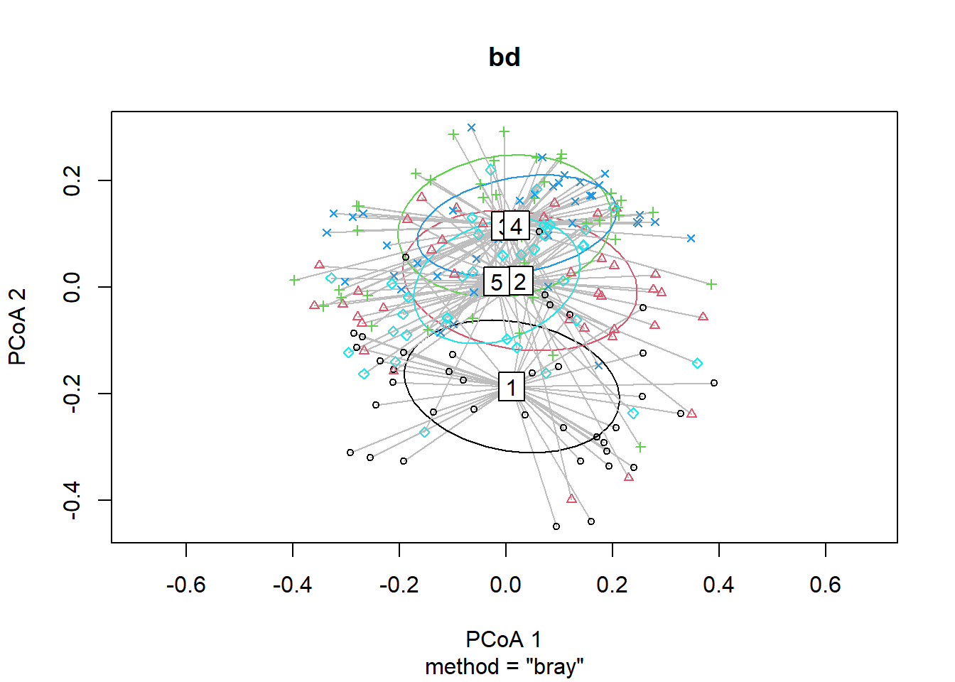
boxplot(bd)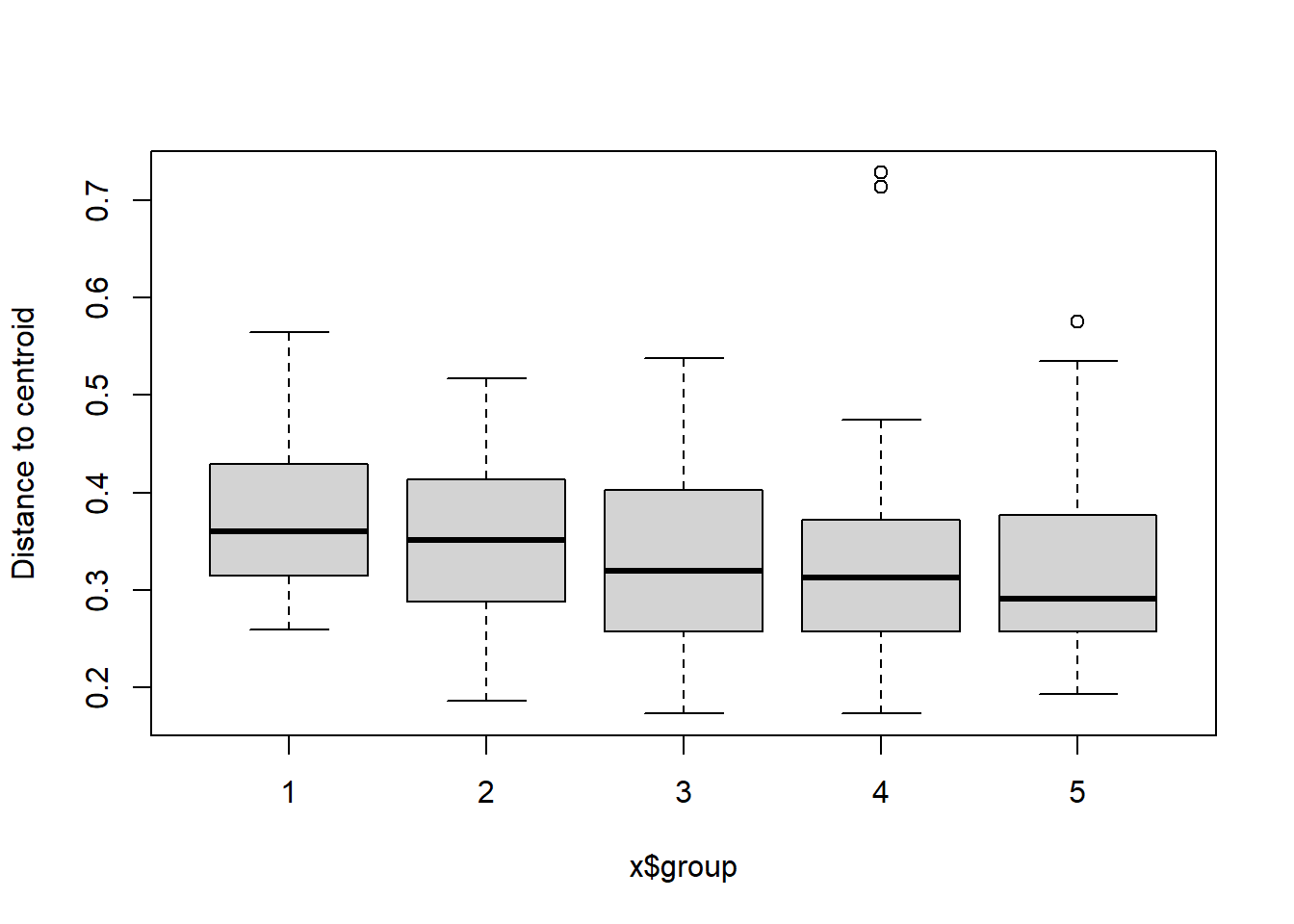
Region group
#Region
bd<-betadisper(trawl_dist,ME_group_data$REGION_NEW)
bd
##
## Homogeneity of multivariate dispersions
##
## Call: betadisper(d = trawl_dist, group = ME_group_data$REGION_NEW)
##
## No. of Positive Eigenvalues: 83
## No. of Negative Eigenvalues: 111
##
## Average distance to median:
## East of Penobscot Bay Penobscot Bay West of Penobscot Bay
## 0.3520 0.3255 0.3840
##
## Eigenvalues for PCoA axes:
## (Showing 8 of 194 eigenvalues)
## PCoA1 PCoA2 PCoA3 PCoA4 PCoA5 PCoA6 PCoA7 PCoA8
## 7.177 4.988 3.828 2.354 1.707 1.515 1.353 1.176anova(bd) ## Analysis of Variance Table
##
## Response: Distances
## Df Sum Sq Mean Sq F value Pr(>F)
## Groups 2 0.09622 0.048109 5.1894 0.006384 **
## Residuals 192 1.77998 0.009271
## ---
## Signif. codes: 0 '***' 0.001 '**' 0.01 '*' 0.05 '.' 0.1 ' ' 1#test based on permutations
permutest(bd)##
## Permutation test for homogeneity of multivariate dispersions
## Permutation: free
## Number of permutations: 999
##
## Response: Distances
## Df Sum Sq Mean Sq F N.Perm Pr(>F)
## Groups 2 0.09622 0.048109 5.1894 999 0.01 **
## Residuals 192 1.77998 0.009271
## ---
## Signif. codes: 0 '***' 0.001 '**' 0.01 '*' 0.05 '.' 0.1 ' ' 1plot(bd, hull=FALSE, ellipse = TRUE) 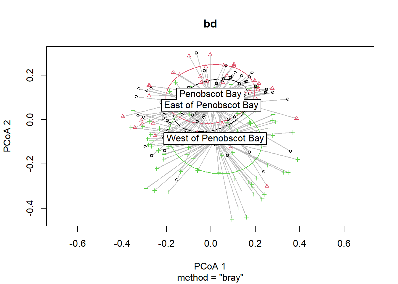
boxplot(bd)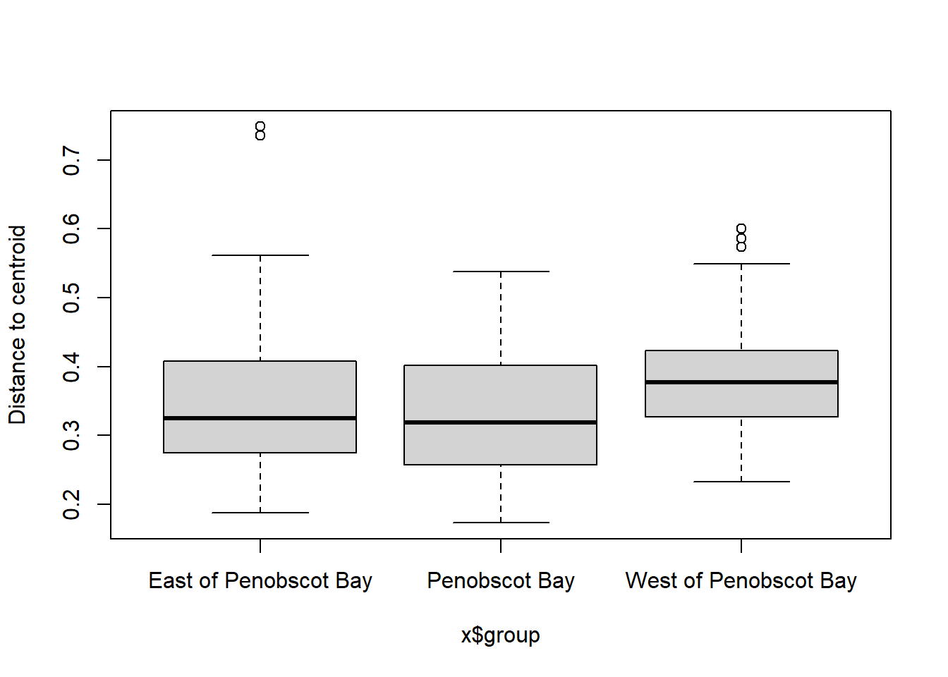
Year
#Year
bd<-betadisper(trawl_dist,ME_group_data$Year)
bd
##
## Homogeneity of multivariate dispersions
##
## Call: betadisper(d = trawl_dist, group = ME_group_data$Year)
##
## No. of Positive Eigenvalues: 83
## No. of Negative Eigenvalues: 111
##
## Average distance to median:
## 2000 2001 2002 2003 2004 2005 2006 2007 2008 2009 2010
## 0.2937 0.3911 0.3688 0.3792 0.4275 0.3783 0.3880 0.4373 0.3760 0.3541 0.3072
## 2011 2012 2013 2014 2015 2016 2017 2018 2019
## 0.3562 0.2519 0.2343 0.2767 0.3180 0.2854 0.2742 0.3512 0.2904
##
## Eigenvalues for PCoA axes:
## (Showing 8 of 194 eigenvalues)
## PCoA1 PCoA2 PCoA3 PCoA4 PCoA5 PCoA6 PCoA7 PCoA8
## 7.177 4.988 3.828 2.354 1.707 1.515 1.353 1.176anova(bd) ## Analysis of Variance Table
##
## Response: Distances
## Df Sum Sq Mean Sq F value Pr(>F)
## Groups 19 0.63018 0.033167 3.6271 2.865e-06 ***
## Residuals 175 1.60025 0.009144
## ---
## Signif. codes: 0 '***' 0.001 '**' 0.01 '*' 0.05 '.' 0.1 ' ' 1#test based on permutations
permutest(bd)##
## Permutation test for homogeneity of multivariate dispersions
## Permutation: free
## Number of permutations: 999
##
## Response: Distances
## Df Sum Sq Mean Sq F N.Perm Pr(>F)
## Groups 19 0.63018 0.033167 3.6271 999 0.001 ***
## Residuals 175 1.60025 0.009144
## ---
## Signif. codes: 0 '***' 0.001 '**' 0.01 '*' 0.05 '.' 0.1 ' ' 1plot(bd, hull=FALSE, ellipse = TRUE)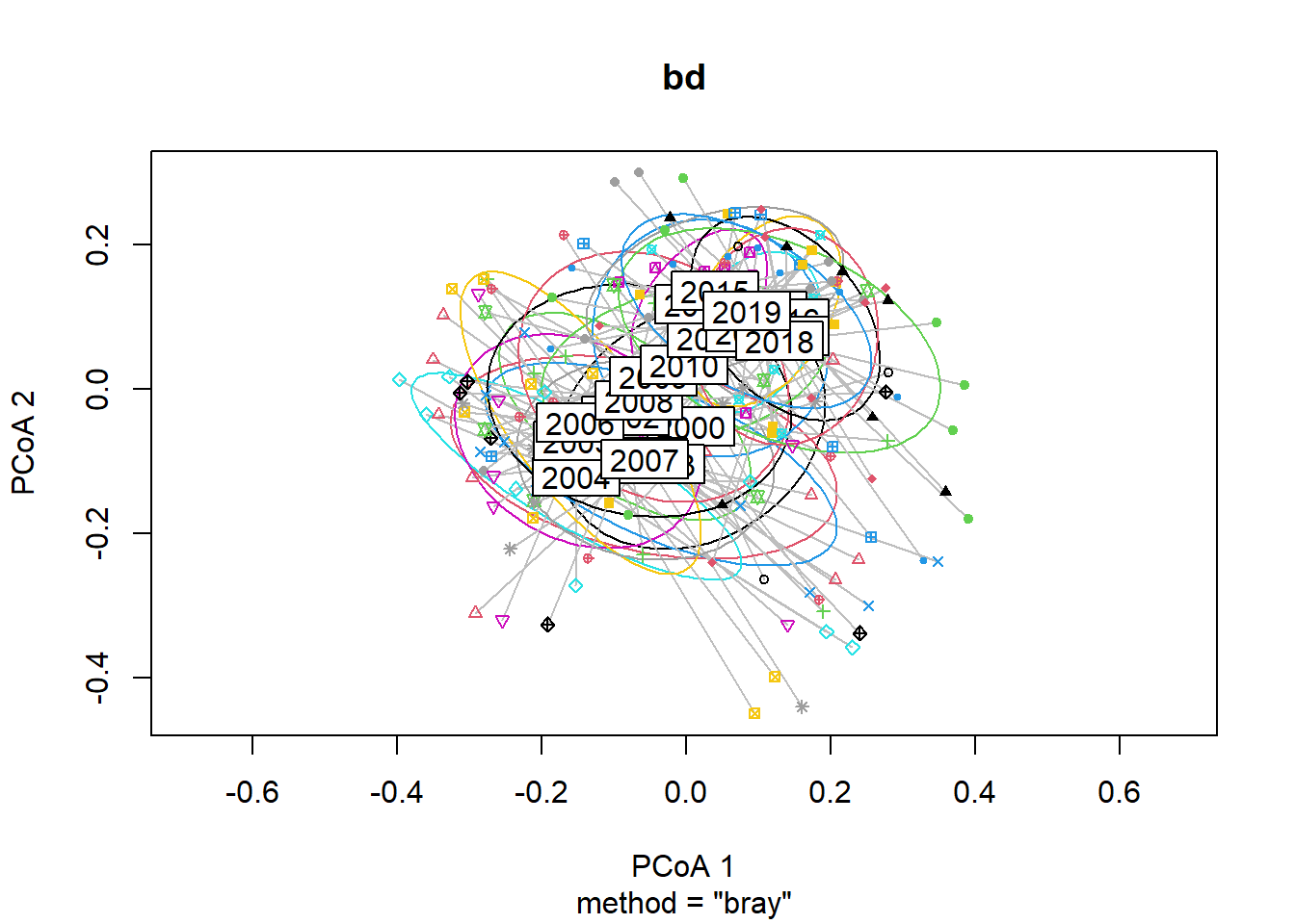
boxplot(bd)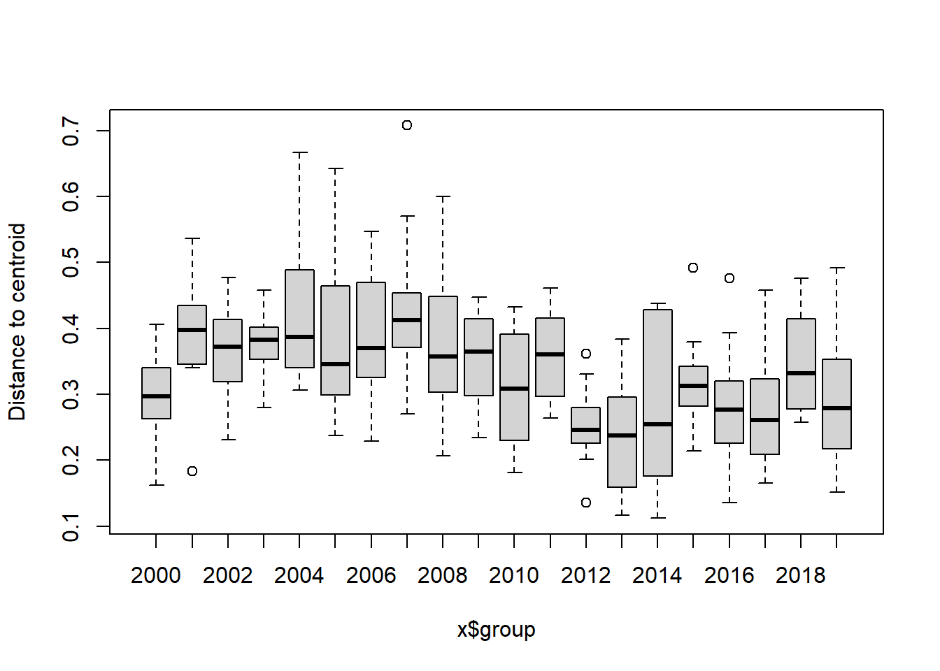
Year block
#Year blocks
bd<-betadisper(trawl_dist,ME_group_data$YEAR_GROUPS)
bd
##
## Homogeneity of multivariate dispersions
##
## Call: betadisper(d = trawl_dist, group = ME_group_data$YEAR_GROUPS)
##
## No. of Positive Eigenvalues: 83
## No. of Negative Eigenvalues: 111
##
## Average distance to median:
## 2000-2004 2005-2009 2010-2014 2015-2019
## 0.3991 0.4011 0.3045 0.3175
##
## Eigenvalues for PCoA axes:
## (Showing 8 of 194 eigenvalues)
## PCoA1 PCoA2 PCoA3 PCoA4 PCoA5 PCoA6 PCoA7 PCoA8
## 7.177 4.988 3.828 2.354 1.707 1.515 1.353 1.176anova(bd) ## Analysis of Variance Table
##
## Response: Distances
## Df Sum Sq Mean Sq F value Pr(>F)
## Groups 3 0.39156 0.130521 14.687 1.205e-08 ***
## Residuals 191 1.69735 0.008887
## ---
## Signif. codes: 0 '***' 0.001 '**' 0.01 '*' 0.05 '.' 0.1 ' ' 1#test based on permutations
permutest(bd)##
## Permutation test for homogeneity of multivariate dispersions
## Permutation: free
## Number of permutations: 999
##
## Response: Distances
## Df Sum Sq Mean Sq F N.Perm Pr(>F)
## Groups 3 0.39156 0.130521 14.687 999 0.001 ***
## Residuals 191 1.69735 0.008887
## ---
## Signif. codes: 0 '***' 0.001 '**' 0.01 '*' 0.05 '.' 0.1 ' ' 1plot(bd, hull=FALSE, ellipse = TRUE)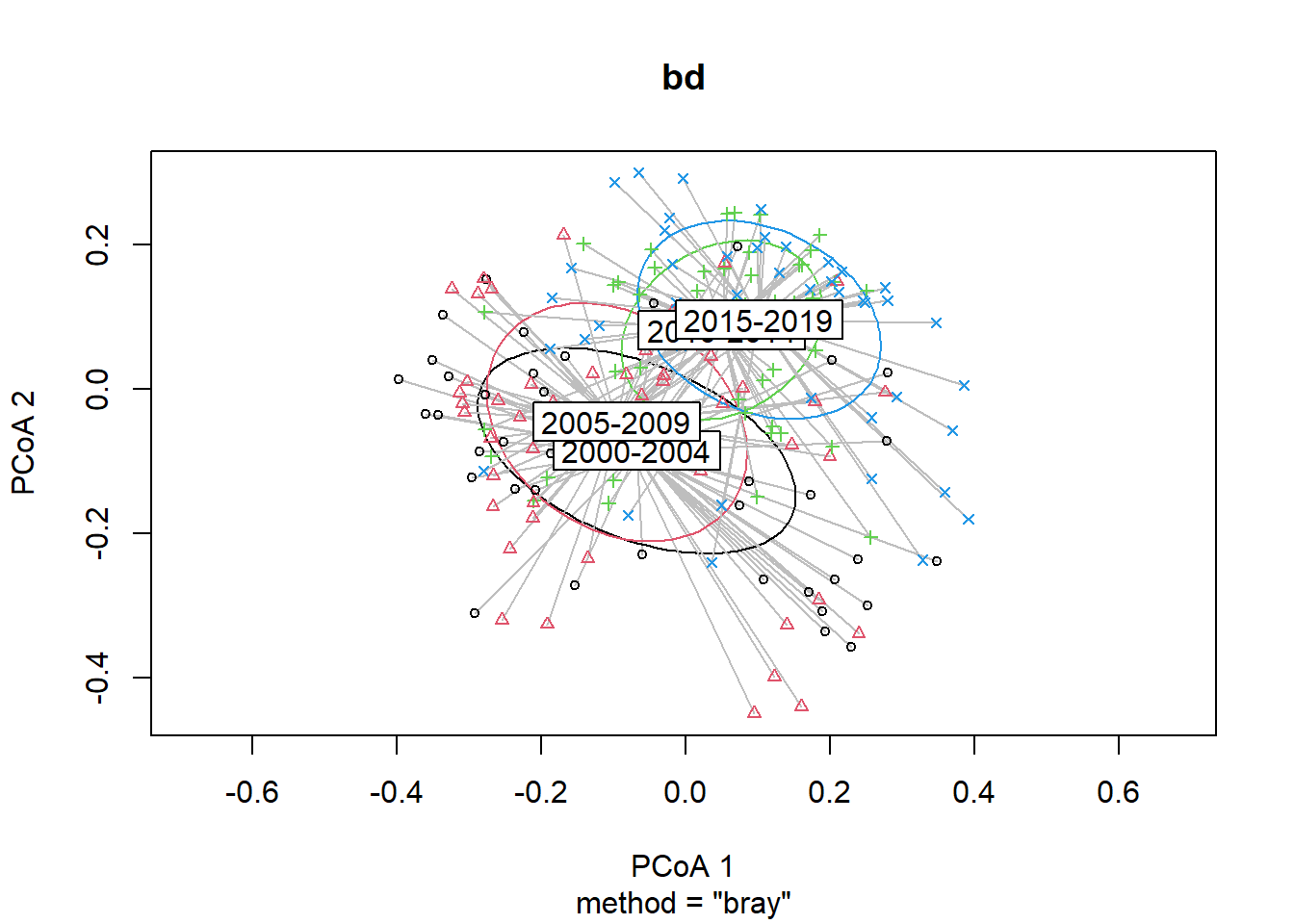
boxplot(bd)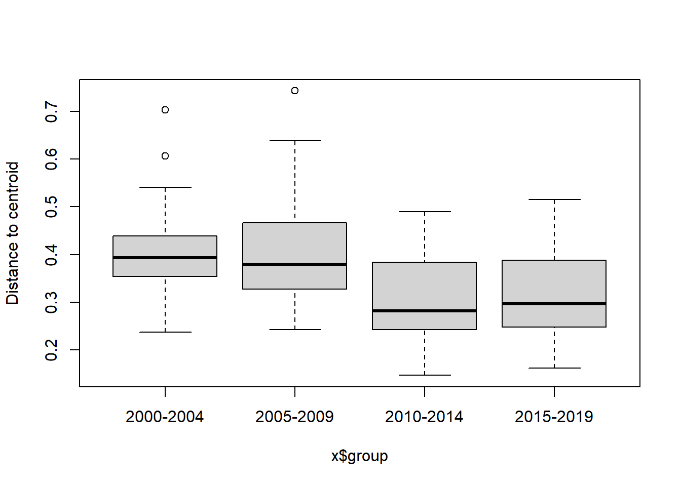
Indicator species analysis
- test if a species if found significantly more in one group compared to another
- all combinations of groups
Region
#see which species are found significantly more in each Region
inv_region<-multipatt(ME_NMDS_data, ME_group_data$Region, func = "r.g", control = how(nperm=999))
summary(inv_region)
##
## Multilevel pattern analysis
## ---------------------------
##
## Association function: r.g
## Significance level (alpha): 0.05
##
## Total number of species: 50
## Selected number of species: 37
## Number of species associated to 1 group: 17
## Number of species associated to 2 groups: 15
## Number of species associated to 3 groups: 3
## Number of species associated to 4 groups: 2
##
## List of species associated to each combination:
##
## Group 1 #sps. 9
## stat p.value
## flounder.yellowtail 0.789 0.001 ***
## cod.atlantic 0.517 0.001 ***
## haddock 0.412 0.001 ***
## dogfish.spiny 0.379 0.001 ***
## hake.atlantic.red 0.280 0.003 **
## mackerel.atlantic 0.219 0.024 *
## squid.long.finned 0.211 0.030 *
## butterfish 0.210 0.037 *
## redfish.acadian.ocean.perch 0.205 0.001 ***
##
## Group 2 #sps. 4
## stat p.value
## alewife 0.455 0.001 ***
## crab.northern.stone 0.354 0.001 ***
## smelt.rainbow 0.340 0.001 ***
## sturgeon.atlantic 0.256 0.008 **
##
## Group 4 #sps. 3
## stat p.value
## cucumber.sea 0.224 0.004 **
## scallop.sea 0.205 0.040 *
## crab.green 0.172 0.008 **
##
## Group 5 #sps. 1
## stat p.value
## flounder.winter 0.646 0.001 ***
##
## Group 1+2 #sps. 7
## stat p.value
## plaice.american..dab. 0.676 0.001 ***
## shad.american 0.401 0.001 ***
## cunner 0.380 0.001 ***
## sculpin.longhorn 0.334 0.001 ***
## herring.blueback 0.305 0.001 ***
## monkfish 0.291 0.003 **
## crab.red 0.219 0.005 **
##
## Group 1+5 #sps. 6
## stat p.value
## sea.raven 0.533 0.001 ***
## skate.little 0.477 0.001 ***
## pout.ocean 0.460 0.001 ***
## skate.smooth 0.299 0.002 **
## skate.winter 0.229 0.015 *
## flounder.atlantic.witch..gray.sole. 0.215 0.029 *
##
## Group 3+4 #sps. 1
## stat p.value
## crab.atlantic.rock 0.347 0.001 ***
##
## Group 4+5 #sps. 1
## stat p.value
## crab.jonah 0.339 0.001 ***
##
## Group 1+2+5 #sps. 1
## stat p.value
## skate.thorny 0.297 0.001 ***
##
## Group 2+3+4 #sps. 1
## stat p.value
## herring.atlantic 0.319 0.001 ***
##
## Group 3+4+5 #sps. 1
## stat p.value
## halibut.atlantic 0.26 0.004 **
##
## Group 1+2+3+4 #sps. 1
## stat p.value
## hake.silver..whiting. 0.209 0.036 *
##
## Group 2+3+4+5 #sps. 1
## stat p.value
## lobster.american 0.329 0.001 ***
## ---
## Signif. codes: 0 '***' 0.001 '**' 0.01 '*' 0.05 '.' 0.1 ' ' 1Year block
#see which species are found significantly more in each Region
inv_year<-multipatt(ME_NMDS_data, ME_group_data$YEAR_GROUPS, func = "r.g", control = how(nperm=999))
summary(inv_year)
##
## Multilevel pattern analysis
## ---------------------------
##
## Association function: r.g
## Significance level (alpha): 0.05
##
## Total number of species: 50
## Selected number of species: 23
## Number of species associated to 1 group: 13
## Number of species associated to 2 groups: 8
## Number of species associated to 3 groups: 2
##
## List of species associated to each combination:
##
## Group 2000-2004 #sps. 6
## stat p.value
## scallop.sea 0.374 0.001 ***
## skate.little 0.321 0.001 ***
## sea.raven 0.318 0.001 ***
## monkfish 0.281 0.001 ***
## skate.winter 0.236 0.004 **
## scup 0.202 0.001 ***
##
## Group 2005-2009 #sps. 3
## stat p.value
## plaice.american..dab. 0.269 0.001 ***
## wolffish.atlantic 0.207 0.023 *
## squid.short.finned 0.184 0.012 *
##
## Group 2010-2014 #sps. 1
## stat p.value
## crab.green 0.152 0.009 **
##
## Group 2015-2019 #sps. 3
## stat p.value
## hake.atlantic.red 0.337 0.001 ***
## haddock 0.305 0.001 ***
## hake.white 0.303 0.001 ***
##
## Group 2000-2004+2005-2009 #sps. 5
## stat p.value
## sculpin.longhorn 0.436 0.001 ***
## menhaden.atlantic 0.233 0.007 **
## smelt.rainbow 0.213 0.014 *
## skate.thorny 0.206 0.018 *
## lumpfish 0.171 0.031 *
##
## Group 2010-2014+2015-2019 #sps. 3
## stat p.value
## lobster.american 0.499 0.001 ***
## skate.barndoor 0.231 0.009 **
## halibut.atlantic 0.230 0.006 **
##
## Group 2000-2004+2005-2009+2015-2019 #sps. 1
## stat p.value
## crab.jonah 0.286 0.001 ***
##
## Group 2000-2004+2010-2014+2015-2019 #sps. 1
## stat p.value
## hake.silver..whiting. 0.279 0.001 ***
## ---
## Signif. codes: 0 '***' 0.001 '**' 0.01 '*' 0.05 '.' 0.1 ' ' 1Data- Abundance of top 50 species
- average across depth strata using the NOAA IEA technical document
- calculate dissimilarity matrix with Bray-Curtis distances
Analysis of similarity (Anosim)
- tests statistically whether there is a significant difference between two or more groups
- works by testing if distances between groups are greater than within groups
- significant values mean that there is a statistically significant difference in the communities between the groups
- R statistic closer to 1 is more dissimilar
Region
#region
ano_region<- anosim(trawl_dist, trawl_data_arrange$Region, permutations = 999)
ano_region #regions are statistically different communities
##
## Call:
## anosim(x = trawl_dist, grouping = trawl_data_arrange$Region, permutations = 999)
## Dissimilarity: bray
##
## ANOSIM statistic R: 0.2496
## Significance: 0.001
##
## Permutation: free
## Number of permutations: 999summary(ano_region)##
## Call:
## anosim(x = trawl_dist, grouping = trawl_data_arrange$Region, permutations = 999)
## Dissimilarity: bray
##
## ANOSIM statistic R: 0.2496
## Significance: 0.001
##
## Permutation: free
## Number of permutations: 999
##
## Upper quantiles of permutations (null model):
## 90% 95% 97.5% 99%
## 0.0114 0.0168 0.0203 0.0246
##
## Dissimilarity ranks between and within classes:
## 0% 25% 50% 75% 100% N
## Between 1 5233.25 10146.5 14731.75 18914 15210
## 1 180 4859.00 8326.0 12478.00 18597 741
## 2 11 3799.00 7713.0 12229.00 18750 741
## 3 3 1824.00 4574.0 8570.00 18410 741
## 4 8 2345.00 4632.0 8828.00 18068 741
## 5 89 5749.00 9459.0 13128.00 18915 741plot(ano_region) #regions don't look very different in plot though...confidence bands all overlap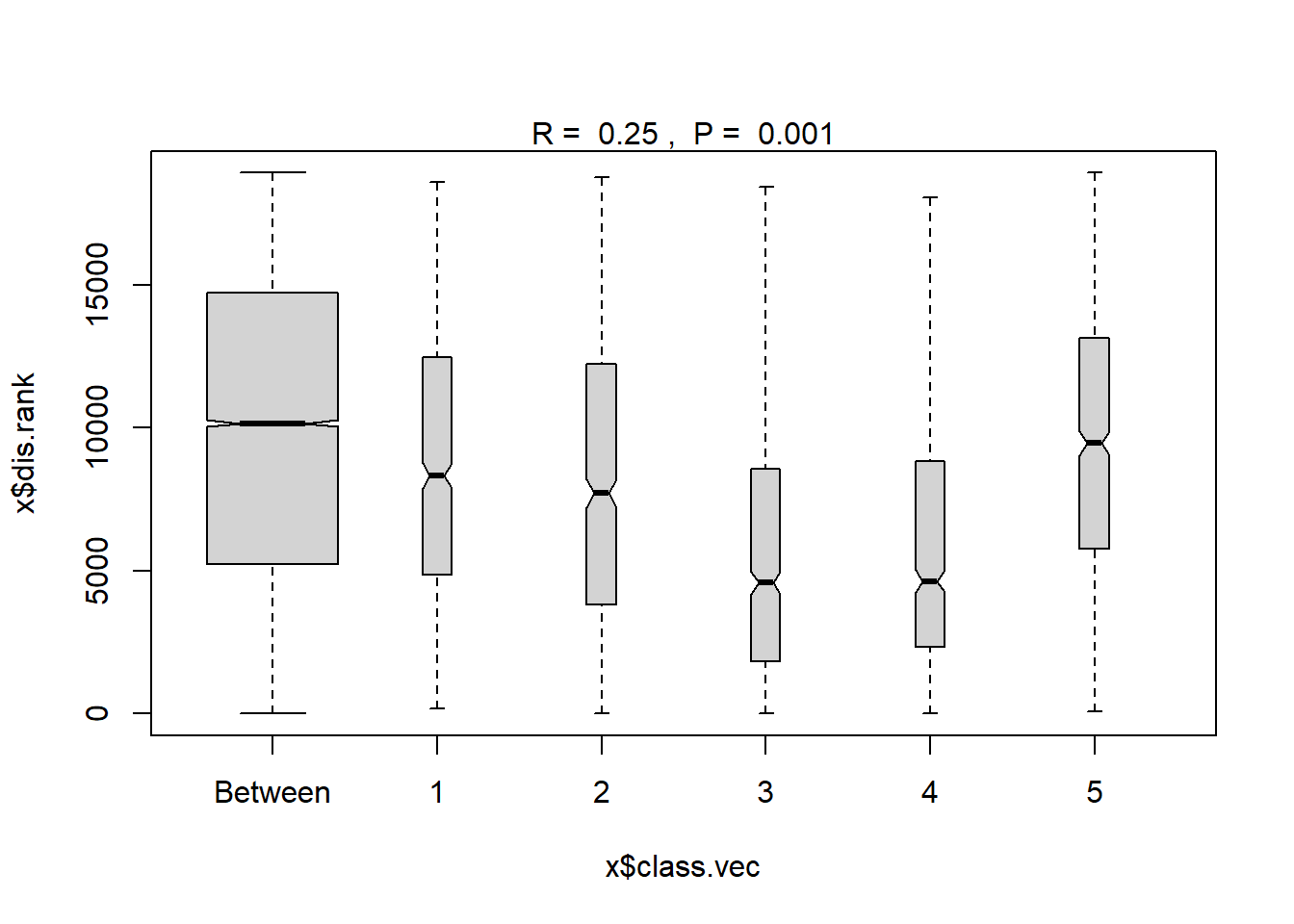
Region grouped
#region
ano_region_groups<- anosim(trawl_dist, trawl_data_arrange$REGION_NEW, permutations = 999)
ano_region_groups #regions are statistically different communities
##
## Call:
## anosim(x = trawl_dist, grouping = trawl_data_arrange$REGION_NEW, permutations = 999)
## Dissimilarity: bray
##
## ANOSIM statistic R: 0.06424
## Significance: 0.001
##
## Permutation: free
## Number of permutations: 999summary(ano_region_groups)##
## Call:
## anosim(x = trawl_dist, grouping = trawl_data_arrange$REGION_NEW, permutations = 999)
## Dissimilarity: bray
##
## ANOSIM statistic R: 0.06424
## Significance: 0.001
##
## Permutation: free
## Number of permutations: 999
##
## Upper quantiles of permutations (null model):
## 90% 95% 97.5% 99%
## 0.0189 0.0253 0.0292 0.0399
##
## Dissimilarity ranks between and within classes:
## 0% 25% 50% 75% 100% N
## Between 1 4889.75 9796.5 14554.25 18912 12168
## East of Penobscot Bay 2 4405.00 9267.0 14203.50 18915 3003
## Penobscot Bay 3 1824.00 4574.0 8570.00 18410 741
## West of Penobscot Bay 11 5623.00 9690.0 13614.00 18836 3003plot(ano_region_groups) #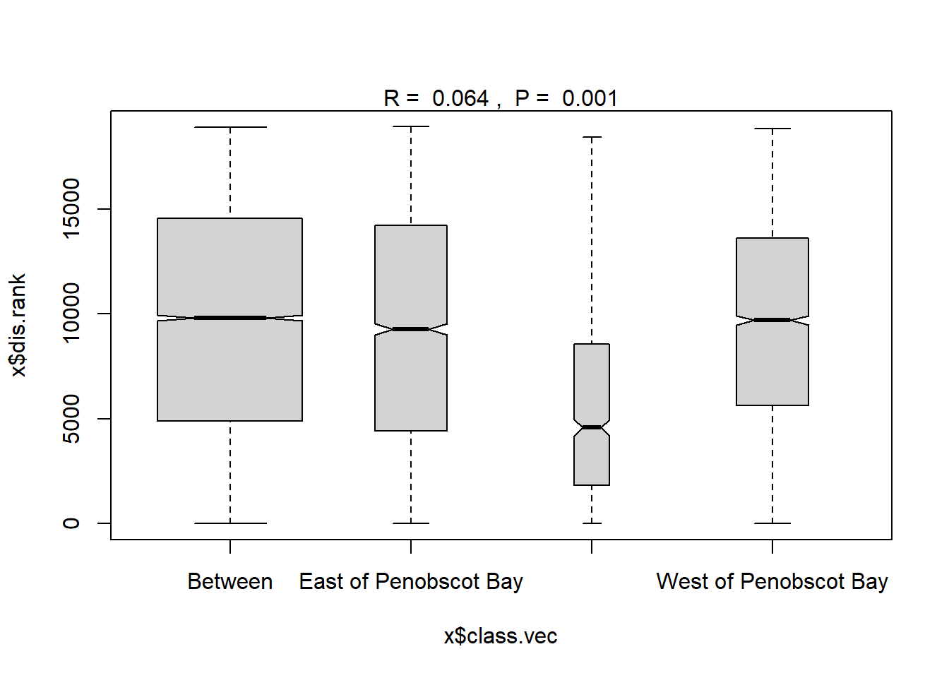
Year
#Time
ano_year<- anosim(trawl_dist, trawl_data_arrange$Year, permutations = 999)
ano_year #years are statistically different communities
##
## Call:
## anosim(x = trawl_dist, grouping = trawl_data_arrange$Year, permutations = 999)
## Dissimilarity: bray
##
## ANOSIM statistic R: 0.1013
## Significance: 0.001
##
## Permutation: free
## Number of permutations: 999summary(ano_year)##
## Call:
## anosim(x = trawl_dist, grouping = trawl_data_arrange$Year, permutations = 999)
## Dissimilarity: bray
##
## ANOSIM statistic R: 0.1013
## Significance: 0.001
##
## Permutation: free
## Number of permutations: 999
##
## Upper quantiles of permutations (null model):
## 90% 95% 97.5% 99%
## 0.0217 0.0278 0.0342 0.0443
##
## Dissimilarity ranks between and within classes:
## 0% 25% 50% 75% 100% N
## Between 1 4784.25 9518.5 14220.75 18915 18050
## 2000 610 4325.50 9209.0 11037.75 12078 10
## 2001 133 5885.00 11954.0 16384.00 18797 45
## 2002 86 7536.00 11592.0 15241.00 18645 45
## 2003 141 3905.00 7997.0 14055.00 18105 45
## 2004 106 6804.00 11918.0 15295.00 18768 45
## 2005 313 8388.00 14193.0 17408.00 18809 45
## 2006 46 4250.00 8796.0 13856.00 18485 45
## 2007 90 8501.00 12175.0 15767.00 18630 45
## 2008 596 7819.00 12987.0 15751.00 17130 45
## 2009 498 4057.00 9114.0 15323.00 18324 45
## 2010 77 2664.00 6096.0 8642.00 15511 45
## 2011 217 5013.00 10282.0 14467.00 18440 45
## 2012 245 3142.00 5065.0 10011.00 15313 45
## 2013 37 1224.00 3824.0 7590.00 13703 45
## 2014 215 2581.00 6406.0 10040.00 16453 45
## 2015 80 3562.00 5921.0 8975.00 17097 45
## 2016 121 2833.00 5330.0 7680.00 15378 45
## 2017 146 2142.00 3464.0 4596.00 7937 45
## 2018 93 5938.00 11633.0 14598.00 17441 45
## 2019 715 3296.00 5494.0 9564.00 15911 45plot(ano_year)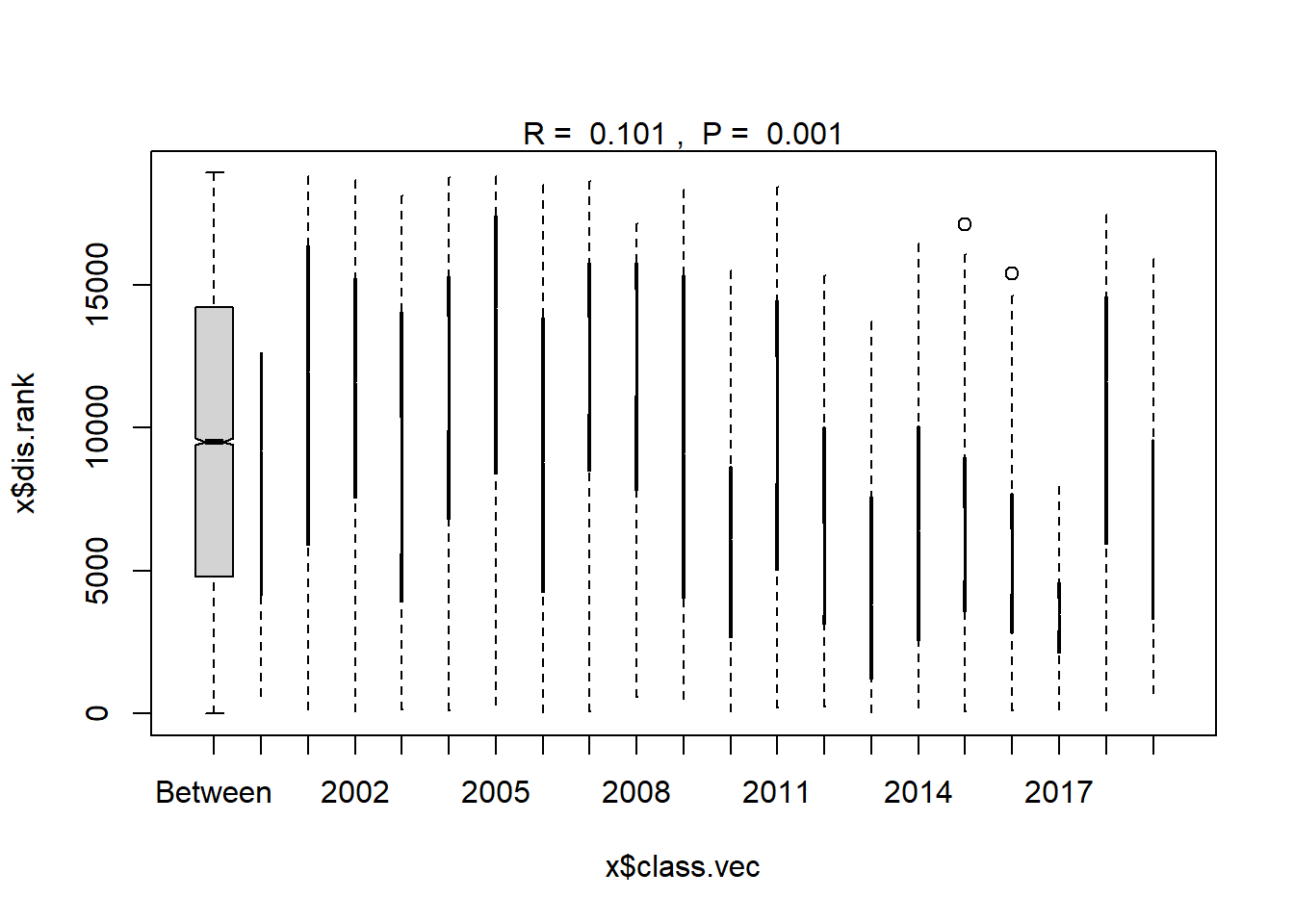
Year blocks
#Year blocks
ano_year_blocks<- anosim(trawl_dist, trawl_data_arrange$YEAR_GROUPS, permutations = 999)
ano_year_blocks #years are statistically different communities
##
## Call:
## anosim(x = trawl_dist, grouping = trawl_data_arrange$YEAR_GROUPS, permutations = 999)
## Dissimilarity: bray
##
## ANOSIM statistic R: 0.1041
## Significance: 0.001
##
## Permutation: free
## Number of permutations: 999summary(ano_year_blocks)##
## Call:
## anosim(x = trawl_dist, grouping = trawl_data_arrange$YEAR_GROUPS, permutations = 999)
## Dissimilarity: bray
##
## ANOSIM statistic R: 0.1041
## Significance: 0.001
##
## Permutation: free
## Number of permutations: 999
##
## Upper quantiles of permutations (null model):
## 90% 95% 97.5% 99%
## 0.0113 0.0165 0.0207 0.0253
##
## Dissimilarity ranks between and within classes:
## 0% 25% 50% 75% 100% N
## Between 1 5042.50 9801.5 14397.75 18914 14250
## 2000-2004 6 5001.25 10216.0 15071.00 18915 990
## 2005-2009 5 6015.00 11985.0 15745.00 18902 1225
## 2010-2014 9 2714.00 6315.0 10776.00 18631 1225
## 2015-2019 11 3387.00 6539.0 10624.00 18493 1225plot(ano_year_blocks)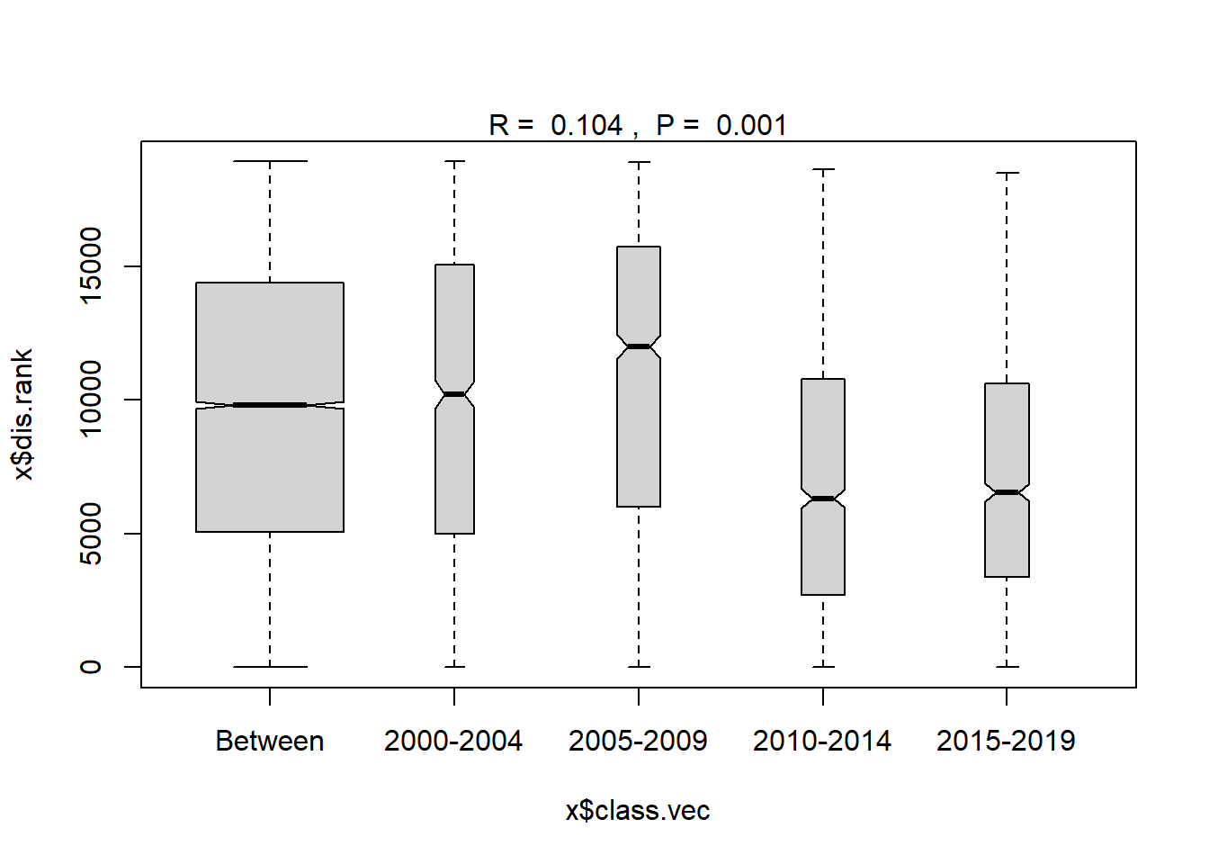
Analysis of variance (Adonis)
- Permanova
- tests whether there is a difference between means of groups
- works by calculating the sum of squares from the centroid of the group
Region
adonis<-adonis2(trawl_dist~Region, data=ME_group_data, by="terms", permutations = 9999)
adonis
## Permutation test for adonis under reduced model
## Terms added sequentially (first to last)
## Permutation: free
## Number of permutations: 9999
##
## adonis2(formula = trawl_dist ~ Region, data = ME_group_data, permutations = 9999, by = "terms")
## Df SumOfSqs R2 F Pr(>F)
## Region 1 1.6434 0.05477 11.183 1e-04 ***
## Residual 193 28.3614 0.94523
## Total 194 30.0048 1.00000
## ---
## Signif. codes: 0 '***' 0.001 '**' 0.01 '*' 0.05 '.' 0.1 ' ' 1summary(adonis)## Df SumOfSqs R2 F
## Min. : 1.0 Min. : 1.643 Min. :0.05477 Min. :11.18
## 1st Qu.: 97.0 1st Qu.:15.002 1st Qu.:0.50000 1st Qu.:11.18
## Median :193.0 Median :28.361 Median :0.94523 Median :11.18
## Mean :129.3 Mean :20.003 Mean :0.66667 Mean :11.18
## 3rd Qu.:193.5 3rd Qu.:29.183 3rd Qu.:0.97261 3rd Qu.:11.18
## Max. :194.0 Max. :30.005 Max. :1.00000 Max. :11.18
## NA's :2
## Pr(>F)
## Min. :1e-04
## 1st Qu.:1e-04
## Median :1e-04
## Mean :1e-04
## 3rd Qu.:1e-04
## Max. :1e-04
## NA's :2Year
adonis<-adonis2(trawl_dist~Year, data=ME_group_data, by="terms", permutations = 9999)
adonis
## Permutation test for adonis under reduced model
## Terms added sequentially (first to last)
## Permutation: free
## Number of permutations: 9999
##
## adonis2(formula = trawl_dist ~ Year, data = ME_group_data, permutations = 9999, by = "terms")
## Df SumOfSqs R2 F Pr(>F)
## Year 1 1.4522 0.0484 9.8159 1e-04 ***
## Residual 193 28.5527 0.9516
## Total 194 30.0048 1.0000
## ---
## Signif. codes: 0 '***' 0.001 '**' 0.01 '*' 0.05 '.' 0.1 ' ' 1summary(adonis)## Df SumOfSqs R2 F
## Min. : 1.0 Min. : 1.452 Min. :0.0484 Min. :9.816
## 1st Qu.: 97.0 1st Qu.:15.002 1st Qu.:0.5000 1st Qu.:9.816
## Median :193.0 Median :28.553 Median :0.9516 Median :9.816
## Mean :129.3 Mean :20.003 Mean :0.6667 Mean :9.816
## 3rd Qu.:193.5 3rd Qu.:29.279 3rd Qu.:0.9758 3rd Qu.:9.816
## Max. :194.0 Max. :30.005 Max. :1.0000 Max. :9.816
## NA's :2
## Pr(>F)
## Min. :1e-04
## 1st Qu.:1e-04
## Median :1e-04
## Mean :1e-04
## 3rd Qu.:1e-04
## Max. :1e-04
## NA's :2Region and Year
adonis<-adonis2(trawl_dist~Region*Year, data=ME_group_data, by="terms", permutations = 9999)
adonis
## Permutation test for adonis under reduced model
## Terms added sequentially (first to last)
## Permutation: free
## Number of permutations: 9999
##
## adonis2(formula = trawl_dist ~ Region * Year, data = ME_group_data, permutations = 9999, by = "terms")
## Df SumOfSqs R2 F Pr(>F)
## Region 1 1.6434 0.05477 11.768 0.0001 ***
## Year 1 1.4522 0.04840 10.399 0.0001 ***
## Region:Year 1 0.2356 0.00785 1.687 0.1256
## Residual 191 26.6737 0.88898
## Total 194 30.0048 1.00000
## ---
## Signif. codes: 0 '***' 0.001 '**' 0.01 '*' 0.05 '.' 0.1 ' ' 1summary(adonis)## Df SumOfSqs R2 F
## Min. : 1.0 Min. : 0.2356 Min. :0.007852 Min. : 1.687
## 1st Qu.: 1.0 1st Qu.: 1.4522 1st Qu.:0.048398 1st Qu.: 6.043
## Median : 1.0 Median : 1.6434 Median :0.054771 Median :10.398
## Mean : 77.6 Mean :12.0019 Mean :0.400000 Mean : 7.951
## 3rd Qu.:191.0 3rd Qu.:26.6737 3rd Qu.:0.888979 3rd Qu.:11.083
## Max. :194.0 Max. :30.0048 Max. :1.000000 Max. :11.768
## NA's :2
## Pr(>F)
## Min. :0.00010
## 1st Qu.:0.00010
## Median :0.00010
## Mean :0.04193
## 3rd Qu.:0.06285
## Max. :0.12560
## NA's :2Year block
#with year blocks
adonis<-adonis2(trawl_dist~YEAR_GROUPS, data=ME_group_data, by="terms", permutations = 9999)
adonis
## Permutation test for adonis under reduced model
## Terms added sequentially (first to last)
## Permutation: free
## Number of permutations: 9999
##
## adonis2(formula = trawl_dist ~ YEAR_GROUPS, data = ME_group_data, permutations = 9999, by = "terms")
## Df SumOfSqs R2 F Pr(>F)
## YEAR_GROUPS 3 2.6412 0.08803 6.1453 1e-04 ***
## Residual 191 27.3636 0.91197
## Total 194 30.0048 1.00000
## ---
## Signif. codes: 0 '***' 0.001 '**' 0.01 '*' 0.05 '.' 0.1 ' ' 1summary(adonis)## Df SumOfSqs R2 F
## Min. : 3.0 Min. : 2.641 Min. :0.08803 Min. :6.145
## 1st Qu.: 97.0 1st Qu.:15.002 1st Qu.:0.50000 1st Qu.:6.145
## Median :191.0 Median :27.364 Median :0.91197 Median :6.145
## Mean :129.3 Mean :20.003 Mean :0.66667 Mean :6.145
## 3rd Qu.:192.5 3rd Qu.:28.684 3rd Qu.:0.95599 3rd Qu.:6.145
## Max. :194.0 Max. :30.005 Max. :1.00000 Max. :6.145
## NA's :2
## Pr(>F)
## Min. :1e-04
## 1st Qu.:1e-04
## Median :1e-04
## Mean :1e-04
## 3rd Qu.:1e-04
## Max. :1e-04
## NA's :2Region and year block
#with year blocks
adonis<-adonis2(trawl_dist~Region*YEAR_GROUPS, data=ME_group_data, by="terms", permutations = 9999)
adonis
## Permutation test for adonis under reduced model
## Terms added sequentially (first to last)
## Permutation: free
## Number of permutations: 9999
##
## adonis2(formula = trawl_dist ~ Region * YEAR_GROUPS, data = ME_group_data, permutations = 9999, by = "terms")
## Df SumOfSqs R2 F Pr(>F)
## Region 1 1.6434 0.05477 12.1987 0.0001 ***
## YEAR_GROUPS 3 2.6412 0.08803 6.5351 0.0001 ***
## Region:YEAR_GROUPS 3 0.5275 0.01758 1.3051 0.1818
## Residual 187 25.1927 0.83962
## Total 194 30.0048 1.00000
## ---
## Signif. codes: 0 '***' 0.001 '**' 0.01 '*' 0.05 '.' 0.1 ' ' 1summary(adonis)## Df SumOfSqs R2 F
## Min. : 1.0 Min. : 0.5275 Min. :0.01758 Min. : 1.305
## 1st Qu.: 3.0 1st Qu.: 1.6434 1st Qu.:0.05477 1st Qu.: 3.920
## Median : 3.0 Median : 2.6412 Median :0.08803 Median : 6.535
## Mean : 77.6 Mean :12.0019 Mean :0.40000 Mean : 6.680
## 3rd Qu.:187.0 3rd Qu.:25.1927 3rd Qu.:0.83962 3rd Qu.: 9.367
## Max. :194.0 Max. :30.0048 Max. :1.00000 Max. :12.199
## NA's :2
## Pr(>F)
## Min. :0.00010
## 1st Qu.:0.00010
## Median :0.00010
## Mean :0.06067
## 3rd Qu.:0.09095
## Max. :0.18180
## NA's :2Region groups
#with year blocks
adonis<-adonis2(trawl_dist~REGION_NEW, data=ME_group_data, by="terms", permutations = 9999)
adonis
## Permutation test for adonis under reduced model
## Terms added sequentially (first to last)
## Permutation: free
## Number of permutations: 9999
##
## adonis2(formula = trawl_dist ~ REGION_NEW, data = ME_group_data, permutations = 9999, by = "terms")
## Df SumOfSqs R2 F Pr(>F)
## REGION_NEW 2 2.6907 0.08968 9.457 1e-04 ***
## Residual 192 27.3141 0.91032
## Total 194 30.0048 1.00000
## ---
## Signif. codes: 0 '***' 0.001 '**' 0.01 '*' 0.05 '.' 0.1 ' ' 1summary(adonis)## Df SumOfSqs R2 F
## Min. : 2.0 Min. : 2.691 Min. :0.08968 Min. :9.457
## 1st Qu.: 97.0 1st Qu.:15.002 1st Qu.:0.50000 1st Qu.:9.457
## Median :192.0 Median :27.314 Median :0.91032 Median :9.457
## Mean :129.3 Mean :20.003 Mean :0.66667 Mean :9.457
## 3rd Qu.:193.0 3rd Qu.:28.659 3rd Qu.:0.95516 3rd Qu.:9.457
## Max. :194.0 Max. :30.005 Max. :1.00000 Max. :9.457
## NA's :2
## Pr(>F)
## Min. :1e-04
## 1st Qu.:1e-04
## Median :1e-04
## Mean :1e-04
## 3rd Qu.:1e-04
## Max. :1e-04
## NA's :2Region groups and year block
#with year blocks
adonis<-adonis2(trawl_dist~REGION_NEW*YEAR_GROUPS, data=ME_group_data, by="terms", permutations = 9999)
adonis
## Permutation test for adonis under reduced model
## Terms added sequentially (first to last)
## Permutation: free
## Number of permutations: 9999
##
## adonis2(formula = trawl_dist ~ REGION_NEW * YEAR_GROUPS, data = ME_group_data, permutations = 9999, by = "terms")
## Df SumOfSqs R2 F Pr(>F)
## REGION_NEW 2 2.6907 0.08968 10.3234 0.0001 ***
## YEAR_GROUPS 3 2.6412 0.08803 6.7557 0.0001 ***
## REGION_NEW:YEAR_GROUPS 6 0.8239 0.02746 1.0537 0.3749
## Residual 183 23.8489 0.79484
## Total 194 30.0048 1.00000
## ---
## Signif. codes: 0 '***' 0.001 '**' 0.01 '*' 0.05 '.' 0.1 ' ' 1summary(adonis)## Df SumOfSqs R2 F
## Min. : 2.0 Min. : 0.8239 Min. :0.02746 Min. : 1.054
## 1st Qu.: 3.0 1st Qu.: 2.6412 1st Qu.:0.08803 1st Qu.: 3.905
## Median : 6.0 Median : 2.6907 Median :0.08968 Median : 6.756
## Mean : 77.6 Mean :12.0019 Mean :0.40000 Mean : 6.044
## 3rd Qu.:183.0 3rd Qu.:23.8489 3rd Qu.:0.79484 3rd Qu.: 8.540
## Max. :194.0 Max. :30.0048 Max. :1.00000 Max. :10.323
## NA's :2
## Pr(>F)
## Min. :0.0001
## 1st Qu.:0.0001
## Median :0.0001
## Mean :0.1250
## 3rd Qu.:0.1875
## Max. :0.3749
## NA's :2Pairwise
- Vegan does not have a function for this, but I found a wrapper that seems frequently used on github
- select groups to test, one pair at a time
- Adjust p-values for multiple tests
Region
#pair-wise test to see what is different
pair<-pairwise.adonis2(trawl_dist~Region, data=ME_group_data, by="terms", permutations = 9999)
summary(pair)
## Length Class Mode
## parent_call 1 -none- character
## 1_vs_2 6 anova list
## 1_vs_3 6 anova list
## 1_vs_4 6 anova list
## 1_vs_5 6 anova list
## 2_vs_3 6 anova list
## 2_vs_4 6 anova list
## 2_vs_5 6 anova list
## 3_vs_4 6 anova list
## 3_vs_5 6 anova list
## 4_vs_5 6 anova listpair #shows all the regions are significantly different except 3 and 4## $parent_call
## [1] "trawl_dist ~ Region , strata = Null"
##
## $`1_vs_2`
## Permutation: free
## Number of permutations: 9999
##
## Terms added sequentially (first to last)
##
## Df SumsOfSqs MeanSqs F.Model R2 Pr(>F)
## Region 1 1.5395 1.53954 11.375 0.13019 1e-04 ***
## Residuals 76 10.2859 0.13534 0.86981
## Total 77 11.8254 1.00000
## ---
## Signif. codes: 0 '***' 0.001 '**' 0.01 '*' 0.05 '.' 0.1 ' ' 1
##
## $`1_vs_3`
## Permutation: free
## Number of permutations: 9999
##
## Terms added sequentially (first to last)
##
## Df SumsOfSqs MeanSqs F.Model R2 Pr(>F)
## Region 1 2.744 2.7440 23.553 0.23659 1e-04 ***
## Residuals 76 8.854 0.1165 0.76341
## Total 77 11.598 1.00000
## ---
## Signif. codes: 0 '***' 0.001 '**' 0.01 '*' 0.05 '.' 0.1 ' ' 1
##
## $`1_vs_4`
## Permutation: free
## Number of permutations: 9999
##
## Terms added sequentially (first to last)
##
## Df SumsOfSqs MeanSqs F.Model R2 Pr(>F)
## Region 1 2.7303 2.73027 23.293 0.23459 1e-04 ***
## Residuals 76 8.9083 0.11721 0.76541
## Total 77 11.6386 1.00000
## ---
## Signif. codes: 0 '***' 0.001 '**' 0.01 '*' 0.05 '.' 0.1 ' ' 1
##
## $`1_vs_5`
## Permutation: free
## Number of permutations: 9999
##
## Terms added sequentially (first to last)
##
## Df SumsOfSqs MeanSqs F.Model R2 Pr(>F)
## Region 1 1.4694 1.46937 10.069 0.11699 1e-04 ***
## Residuals 76 11.0907 0.14593 0.88301
## Total 77 12.5601 1.00000
## ---
## Signif. codes: 0 '***' 0.001 '**' 0.01 '*' 0.05 '.' 0.1 ' ' 1
##
## $`2_vs_3`
## Permutation: free
## Number of permutations: 9999
##
## Terms added sequentially (first to last)
##
## Df SumsOfSqs MeanSqs F.Model R2 Pr(>F)
## Region 1 0.5809 0.58091 5.1004 0.06289 0.0014 **
## Residuals 76 8.6560 0.11390 0.93711
## Total 77 9.2369 1.00000
## ---
## Signif. codes: 0 '***' 0.001 '**' 0.01 '*' 0.05 '.' 0.1 ' ' 1
##
## $`2_vs_4`
## Permutation: free
## Number of permutations: 9999
##
## Terms added sequentially (first to last)
##
## Df SumsOfSqs MeanSqs F.Model R2 Pr(>F)
## Region 1 0.5280 0.52797 4.6067 0.05715 0.0016 **
## Residuals 76 8.7103 0.11461 0.94285
## Total 77 9.2383 1.00000
## ---
## Signif. codes: 0 '***' 0.001 '**' 0.01 '*' 0.05 '.' 0.1 ' ' 1
##
## $`2_vs_5`
## Permutation: free
## Number of permutations: 9999
##
## Terms added sequentially (first to last)
##
## Df SumsOfSqs MeanSqs F.Model R2 Pr(>F)
## Region 1 2.0765 2.07654 14.488 0.16011 1e-04 ***
## Residuals 76 10.8927 0.14332 0.83989
## Total 77 12.9692 1.00000
## ---
## Signif. codes: 0 '***' 0.001 '**' 0.01 '*' 0.05 '.' 0.1 ' ' 1
##
## $`3_vs_4`
## Permutation: free
## Number of permutations: 9999
##
## Terms added sequentially (first to last)
##
## Df SumsOfSqs MeanSqs F.Model R2 Pr(>F)
## Region 1 0.0544 0.054402 0.56806 0.00742 0.6859
## Residuals 76 7.2784 0.095769 0.99258
## Total 77 7.3328 1.00000
##
## $`3_vs_5`
## Permutation: free
## Number of permutations: 9999
##
## Terms added sequentially (first to last)
##
## Df SumsOfSqs MeanSqs F.Model R2 Pr(>F)
## Region 1 2.3949 2.39490 19.238 0.202 1e-04 ***
## Residuals 76 9.4608 0.12448 0.798
## Total 77 11.8557 1.000
## ---
## Signif. codes: 0 '***' 0.001 '**' 0.01 '*' 0.05 '.' 0.1 ' ' 1
##
## $`4_vs_5`
## Permutation: free
## Number of permutations: 9999
##
## Terms added sequentially (first to last)
##
## Df SumsOfSqs MeanSqs F.Model R2 Pr(>F)
## Region 1 2.3615 2.3615 18.862 0.19884 1e-04 ***
## Residuals 76 9.5151 0.1252 0.80116
## Total 77 11.8766 1.00000
## ---
## Signif. codes: 0 '***' 0.001 '**' 0.01 '*' 0.05 '.' 0.1 ' ' 1
##
## attr(,"class")
## [1] "pwadstrata" "list"Region groups
#pair-wise test to see what is different
pair<-pairwise.adonis2(trawl_dist~REGION_NEW, data=ME_group_data, by="terms", permutations = 9999)
summary(pair)
## Length Class Mode
## parent_call 1 -none- character
## West of Penobscot Bay_vs_Penobscot Bay 6 anova list
## West of Penobscot Bay_vs_East of Penobscot Bay 6 anova list
## Penobscot Bay_vs_East of Penobscot Bay 6 anova listpair #shows all the regions are significantly different except 3 and 4## $parent_call
## [1] "trawl_dist ~ REGION_NEW , strata = Null"
##
## $`West of Penobscot Bay_vs_Penobscot Bay`
## Permutation: free
## Number of permutations: 9999
##
## Terms added sequentially (first to last)
##
## Df SumsOfSqs MeanSqs F.Model R2 Pr(>F)
## REGION_NEW 1 1.7034 1.70342 12.689 0.09938 1e-04 ***
## Residuals 115 15.4375 0.13424 0.90062
## Total 116 17.1410 1.00000
## ---
## Signif. codes: 0 '***' 0.001 '**' 0.01 '*' 0.05 '.' 0.1 ' ' 1
##
## $`West of Penobscot Bay_vs_East of Penobscot Bay`
## Permutation: free
## Number of permutations: 9999
##
## Terms added sequentially (first to last)
##
## Df SumsOfSqs MeanSqs F.Model R2 Pr(>F)
## REGION_NEW 1 1.4516 1.45157 9.4313 0.05771 1e-04 ***
## Residuals 154 23.7020 0.15391 0.94229
## Total 155 25.1536 1.00000
## ---
## Signif. codes: 0 '***' 0.001 '**' 0.01 '*' 0.05 '.' 0.1 ' ' 1
##
## $`Penobscot Bay_vs_East of Penobscot Bay`
## Permutation: free
## Number of permutations: 9999
##
## Terms added sequentially (first to last)
##
## Df SumsOfSqs MeanSqs F.Model R2 Pr(>F)
## REGION_NEW 1 0.8457 0.84570 6.2792 0.05177 6e-04 ***
## Residuals 115 15.4887 0.13468 0.94823
## Total 116 16.3344 1.00000
## ---
## Signif. codes: 0 '***' 0.001 '**' 0.01 '*' 0.05 '.' 0.1 ' ' 1
##
## attr(,"class")
## [1] "pwadstrata" "list"Year blocks
#pair-wise test to see what is different for year blocks
pair<-pairwise.adonis2(trawl_dist~YEAR_GROUPS, data=ME_group_data, by="terms", permutations = 9999)
summary(pair)
## Length Class Mode
## parent_call 1 -none- character
## 2000-2004_vs_2005-2009 6 anova list
## 2000-2004_vs_2010-2014 6 anova list
## 2000-2004_vs_2015-2019 6 anova list
## 2005-2009_vs_2010-2014 6 anova list
## 2005-2009_vs_2015-2019 6 anova list
## 2010-2014_vs_2015-2019 6 anova listpair## $parent_call
## [1] "trawl_dist ~ YEAR_GROUPS , strata = Null"
##
## $`2000-2004_vs_2005-2009`
## Permutation: free
## Number of permutations: 9999
##
## Terms added sequentially (first to last)
##
## Df SumsOfSqs MeanSqs F.Model R2 Pr(>F)
## YEAR_GROUPS 1 0.575 0.57502 3.3408 0.03468 0.0096 **
## Residuals 93 16.007 0.17212 0.96532
## Total 94 16.582 1.00000
## ---
## Signif. codes: 0 '***' 0.001 '**' 0.01 '*' 0.05 '.' 0.1 ' ' 1
##
## $`2000-2004_vs_2010-2014`
## Permutation: free
## Number of permutations: 9999
##
## Terms added sequentially (first to last)
##
## Df SumsOfSqs MeanSqs F.Model R2 Pr(>F)
## YEAR_GROUPS 1 0.427 0.42699 3.0996 0.03225 0.0182 *
## Residuals 93 12.811 0.13776 0.96775
## Total 94 13.238 1.00000
## ---
## Signif. codes: 0 '***' 0.001 '**' 0.01 '*' 0.05 '.' 0.1 ' ' 1
##
## $`2000-2004_vs_2015-2019`
## Permutation: free
## Number of permutations: 9999
##
## Terms added sequentially (first to last)
##
## Df SumsOfSqs MeanSqs F.Model R2 Pr(>F)
## YEAR_GROUPS 1 1.0762 1.07623 7.7514 0.07694 2e-04 ***
## Residuals 93 12.9125 0.13884 0.92306
## Total 94 13.9887 1.00000
## ---
## Signif. codes: 0 '***' 0.001 '**' 0.01 '*' 0.05 '.' 0.1 ' ' 1
##
## $`2005-2009_vs_2010-2014`
## Permutation: free
## Number of permutations: 9999
##
## Terms added sequentially (first to last)
##
## Df SumsOfSqs MeanSqs F.Model R2 Pr(>F)
## YEAR_GROUPS 1 1.2221 1.22209 8.2875 0.07797 1e-04 ***
## Residuals 98 14.4511 0.14746 0.92203
## Total 99 15.6732 1.00000
## ---
## Signif. codes: 0 '***' 0.001 '**' 0.01 '*' 0.05 '.' 0.1 ' ' 1
##
## $`2005-2009_vs_2015-2019`
## Permutation: free
## Number of permutations: 9999
##
## Terms added sequentially (first to last)
##
## Df SumsOfSqs MeanSqs F.Model R2 Pr(>F)
## YEAR_GROUPS 1 1.5101 1.51011 10.17 0.09402 1e-04 ***
## Residuals 98 14.5522 0.14849 0.90598
## Total 99 16.0623 1.00000
## ---
## Signif. codes: 0 '***' 0.001 '**' 0.01 '*' 0.05 '.' 0.1 ' ' 1
##
## $`2010-2014_vs_2015-2019`
## Permutation: free
## Number of permutations: 9999
##
## Terms added sequentially (first to last)
##
## Df SumsOfSqs MeanSqs F.Model R2 Pr(>F)
## YEAR_GROUPS 1 0.4439 0.44389 3.8305 0.03762 0.0052 **
## Residuals 98 11.3564 0.11588 0.96238
## Total 99 11.8003 1.00000
## ---
## Signif. codes: 0 '***' 0.001 '**' 0.01 '*' 0.05 '.' 0.1 ' ' 1
##
## attr(,"class")
## [1] "pwadstrata" "list"Dispersion
- anosim very sensitive to heterogeneity (Anderson and Walsh 2013)
- Could get false significant results from differences in variance instead of mean
- adonis is less affected by heterogeneity for balanced designs
- PRIMER can deal with dispersion issues, but vegan does not yet
- tests null hypothesis that there is no difference in dispersion between groups
- p-value <0.05 means difference is significant
Region
#betadisper test homogeneity of dispersion among groups
#Region
bd<-betadisper(trawl_dist,ME_group_data$Region)
bd
##
## Homogeneity of multivariate dispersions
##
## Call: betadisper(d = trawl_dist, group = ME_group_data$Region)
##
## No. of Positive Eigenvalues: 74
## No. of Negative Eigenvalues: 120
##
## Average distance to median:
## 1 2 3 4 5
## 0.3571 0.3450 0.2884 0.2939 0.3756
##
## Eigenvalues for PCoA axes:
## (Showing 8 of 194 eigenvalues)
## PCoA1 PCoA2 PCoA3 PCoA4 PCoA5 PCoA6 PCoA7 PCoA8
## 11.115 5.775 2.911 2.701 1.762 1.567 1.432 1.112anova(bd) ## Analysis of Variance Table
##
## Response: Distances
## Df Sum Sq Mean Sq F value Pr(>F)
## Groups 4 0.23632 0.059079 6.2064 0.0001028 ***
## Residuals 190 1.80860 0.009519
## ---
## Signif. codes: 0 '***' 0.001 '**' 0.01 '*' 0.05 '.' 0.1 ' ' 1#test based on permutations
permutest(bd)##
## Permutation test for homogeneity of multivariate dispersions
## Permutation: free
## Number of permutations: 999
##
## Response: Distances
## Df Sum Sq Mean Sq F N.Perm Pr(>F)
## Groups 4 0.23632 0.059079 6.2064 999 0.001 ***
## Residuals 190 1.80860 0.009519
## ---
## Signif. codes: 0 '***' 0.001 '**' 0.01 '*' 0.05 '.' 0.1 ' ' 1plot(bd, hull=FALSE, ellipse = TRUE) 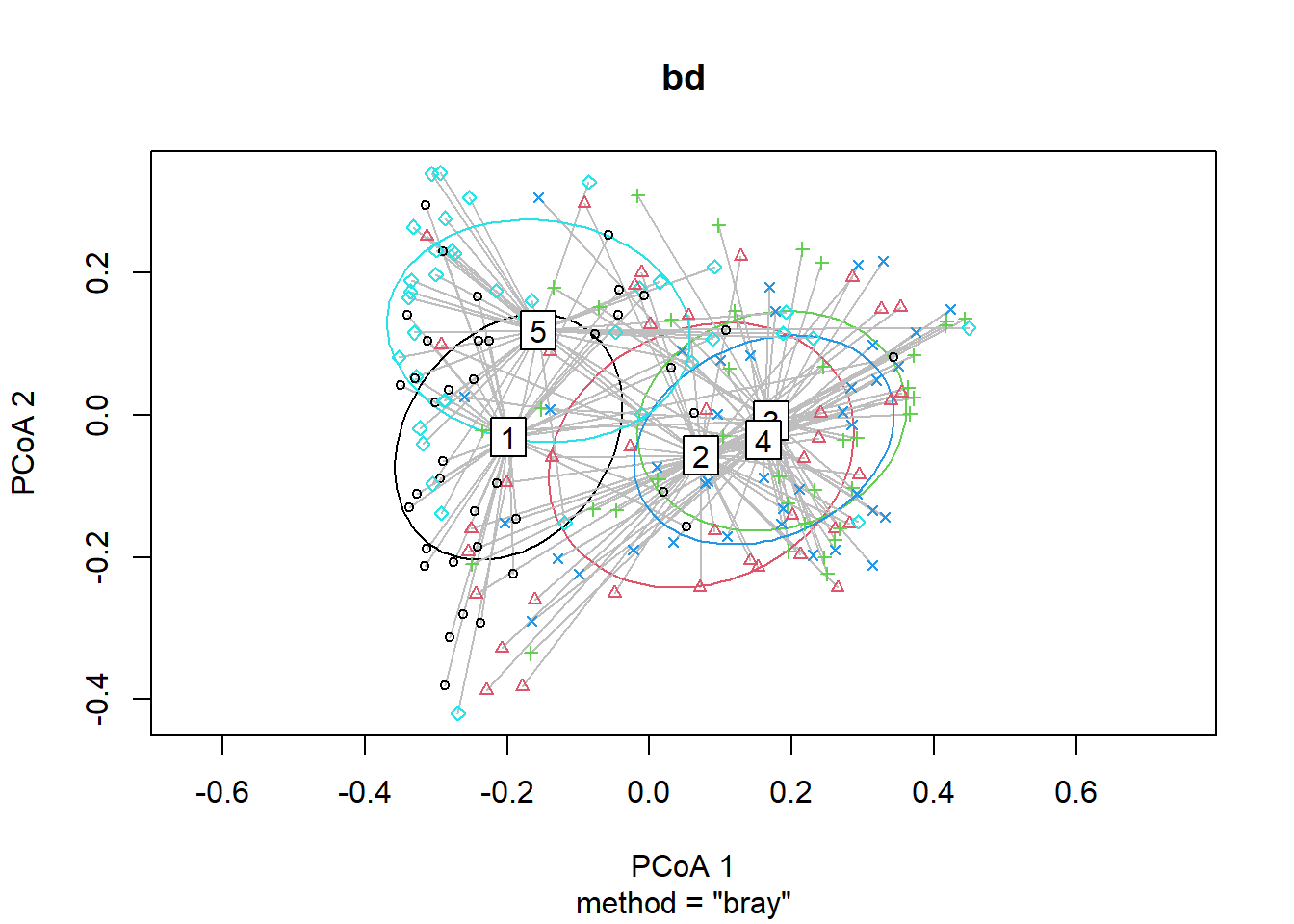
boxplot(bd)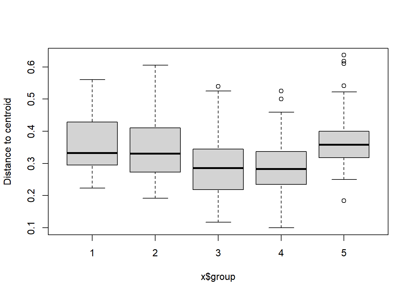
Region group
#Region
bd<-betadisper(trawl_dist,ME_group_data$REGION_NEW)
bd
##
## Homogeneity of multivariate dispersions
##
## Call: betadisper(d = trawl_dist, group = ME_group_data$REGION_NEW)
##
## No. of Positive Eigenvalues: 74
## No. of Negative Eigenvalues: 120
##
## Average distance to median:
## East of Penobscot Bay Penobscot Bay West of Penobscot Bay
## 0.3760 0.2884 0.3811
##
## Eigenvalues for PCoA axes:
## (Showing 8 of 194 eigenvalues)
## PCoA1 PCoA2 PCoA3 PCoA4 PCoA5 PCoA6 PCoA7 PCoA8
## 11.115 5.775 2.911 2.701 1.762 1.567 1.432 1.112anova(bd) ## Analysis of Variance Table
##
## Response: Distances
## Df Sum Sq Mean Sq F value Pr(>F)
## Groups 2 0.2548 0.127399 13.143 4.47e-06 ***
## Residuals 192 1.8611 0.009693
## ---
## Signif. codes: 0 '***' 0.001 '**' 0.01 '*' 0.05 '.' 0.1 ' ' 1#test based on permutations
permutest(bd)##
## Permutation test for homogeneity of multivariate dispersions
## Permutation: free
## Number of permutations: 999
##
## Response: Distances
## Df Sum Sq Mean Sq F N.Perm Pr(>F)
## Groups 2 0.2548 0.127399 13.143 999 0.001 ***
## Residuals 192 1.8611 0.009693
## ---
## Signif. codes: 0 '***' 0.001 '**' 0.01 '*' 0.05 '.' 0.1 ' ' 1plot(bd, hull=FALSE, ellipse = TRUE) 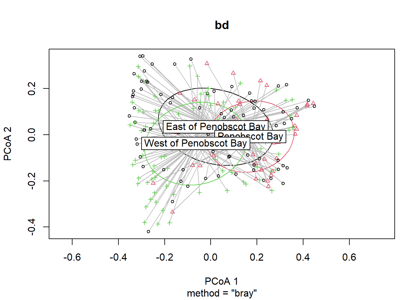
boxplot(bd)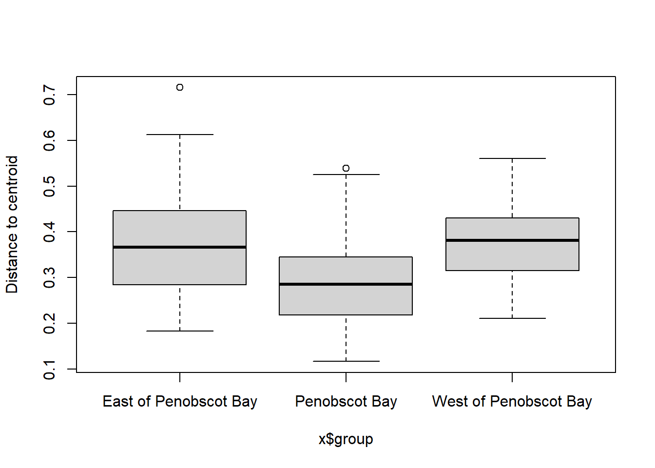
Year
#Year
bd<-betadisper(trawl_dist,ME_group_data$Year)
bd
##
## Homogeneity of multivariate dispersions
##
## Call: betadisper(d = trawl_dist, group = ME_group_data$Year)
##
## No. of Positive Eigenvalues: 74
## No. of Negative Eigenvalues: 120
##
## Average distance to median:
## 2000 2001 2002 2003 2004 2005 2006 2007 2008 2009 2010
## 0.2970 0.3953 0.3954 0.3390 0.3882 0.4162 0.3422 0.3988 0.3927 0.3563 0.2930
## 2011 2012 2013 2014 2015 2016 2017 2018 2019
## 0.3603 0.2943 0.2550 0.3024 0.2983 0.2829 0.2328 0.3707 0.2991
##
## Eigenvalues for PCoA axes:
## (Showing 8 of 194 eigenvalues)
## PCoA1 PCoA2 PCoA3 PCoA4 PCoA5 PCoA6 PCoA7 PCoA8
## 11.115 5.775 2.911 2.701 1.762 1.567 1.432 1.112anova(bd) ## Analysis of Variance Table
##
## Response: Distances
## Df Sum Sq Mean Sq F value Pr(>F)
## Groups 19 0.53872 0.028354 2.275 0.002852 **
## Residuals 175 2.18108 0.012463
## ---
## Signif. codes: 0 '***' 0.001 '**' 0.01 '*' 0.05 '.' 0.1 ' ' 1#test based on permutations
permutest(bd)##
## Permutation test for homogeneity of multivariate dispersions
## Permutation: free
## Number of permutations: 999
##
## Response: Distances
## Df Sum Sq Mean Sq F N.Perm Pr(>F)
## Groups 19 0.53872 0.028354 2.275 999 0.005 **
## Residuals 175 2.18108 0.012463
## ---
## Signif. codes: 0 '***' 0.001 '**' 0.01 '*' 0.05 '.' 0.1 ' ' 1plot(bd, hull=FALSE, ellipse = TRUE)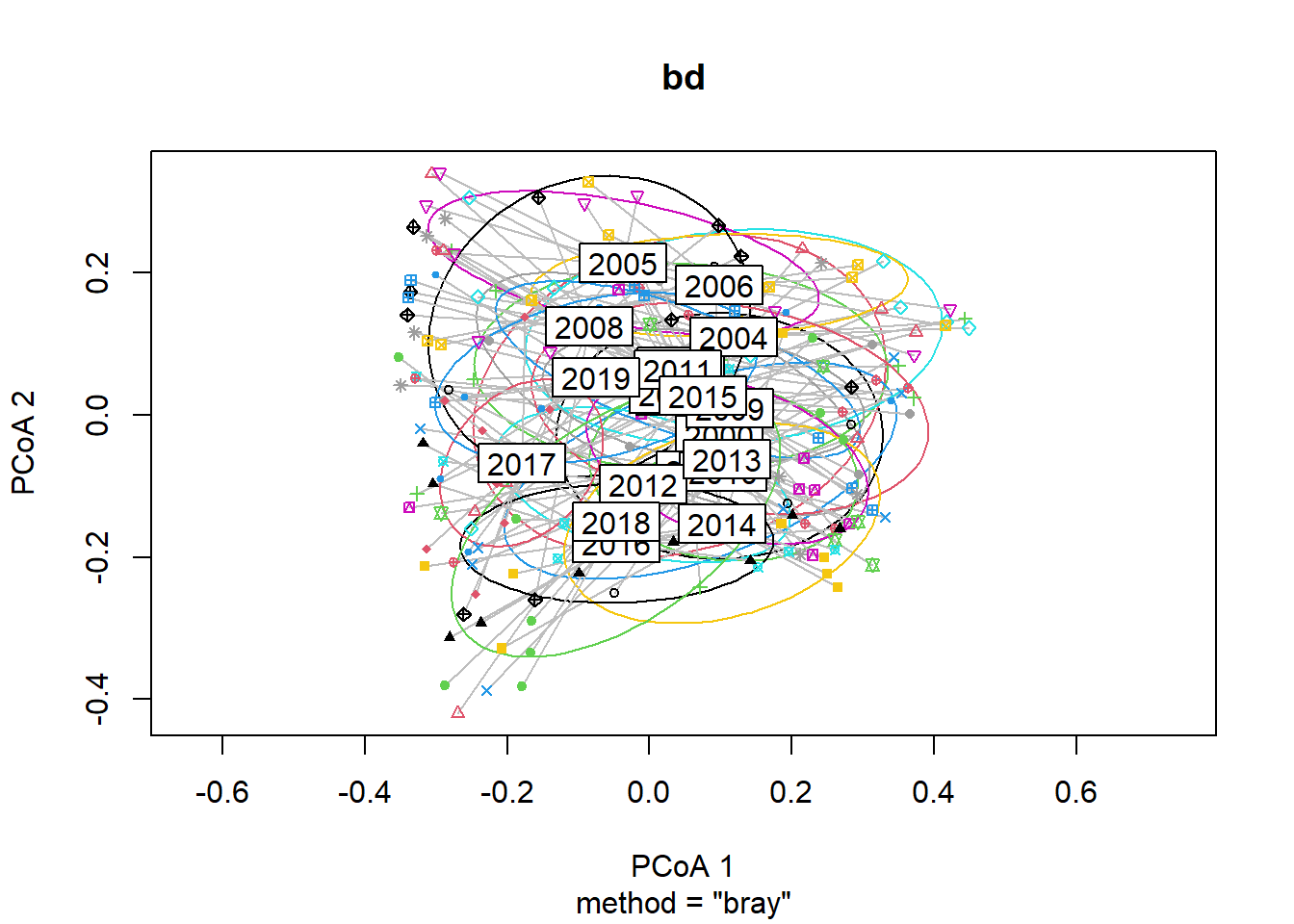
boxplot(bd)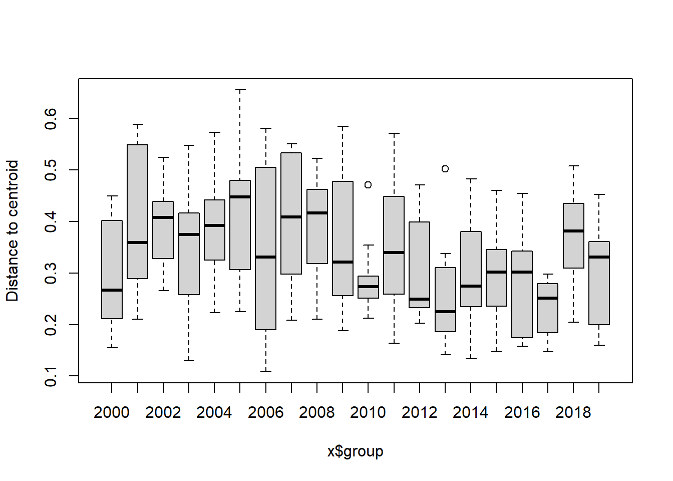
Year block
#Year blocks
bd<-betadisper(trawl_dist,ME_group_data$YEAR_GROUPS)
bd
##
## Homogeneity of multivariate dispersions
##
## Call: betadisper(d = trawl_dist, group = ME_group_data$YEAR_GROUPS)
##
## No. of Positive Eigenvalues: 74
## No. of Negative Eigenvalues: 120
##
## Average distance to median:
## 2000-2004 2005-2009 2010-2014 2015-2019
## 0.3851 0.4073 0.3189 0.3285
##
## Eigenvalues for PCoA axes:
## (Showing 8 of 194 eigenvalues)
## PCoA1 PCoA2 PCoA3 PCoA4 PCoA5 PCoA6 PCoA7 PCoA8
## 11.115 5.775 2.911 2.701 1.762 1.567 1.432 1.112anova(bd) ## Analysis of Variance Table
##
## Response: Distances
## Df Sum Sq Mean Sq F value Pr(>F)
## Groups 3 0.27431 0.091436 8.1518 3.903e-05 ***
## Residuals 191 2.14239 0.011217
## ---
## Signif. codes: 0 '***' 0.001 '**' 0.01 '*' 0.05 '.' 0.1 ' ' 1#test based on permutations
permutest(bd)##
## Permutation test for homogeneity of multivariate dispersions
## Permutation: free
## Number of permutations: 999
##
## Response: Distances
## Df Sum Sq Mean Sq F N.Perm Pr(>F)
## Groups 3 0.27431 0.091436 8.1518 999 0.001 ***
## Residuals 191 2.14239 0.011217
## ---
## Signif. codes: 0 '***' 0.001 '**' 0.01 '*' 0.05 '.' 0.1 ' ' 1plot(bd, hull=FALSE, ellipse = TRUE)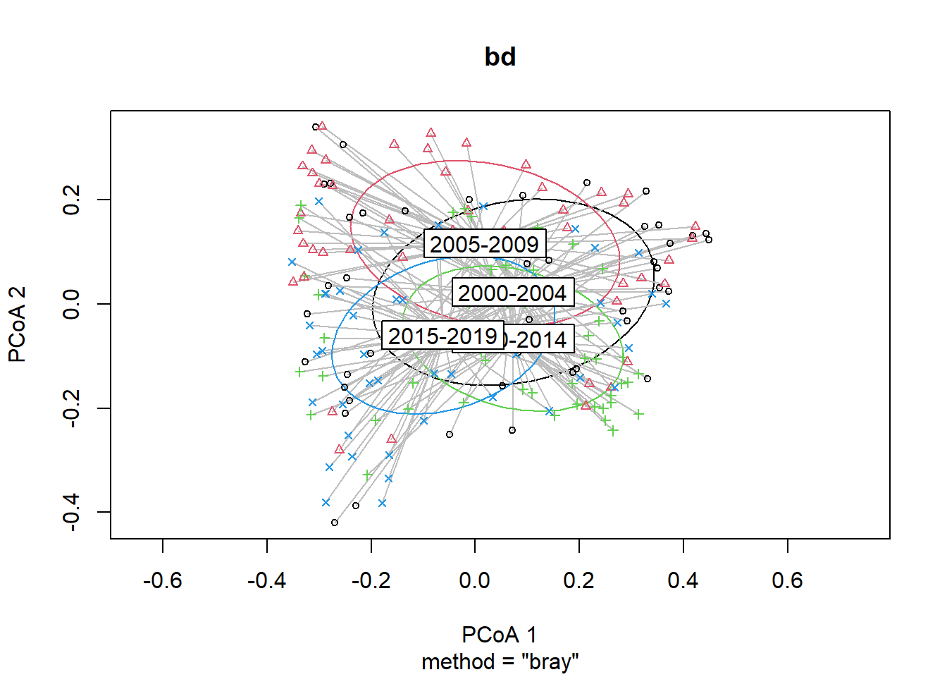
boxplot(bd)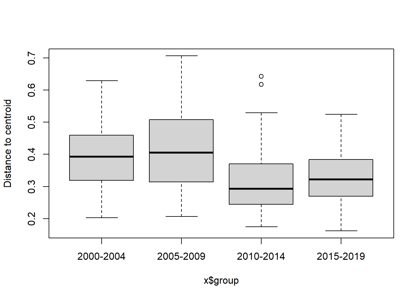
Indicator species analysis
- test if a species if found significantly more in one group compared to another
- all combinations of groups
Region
#see which species are found significantly more in each Region
inv_region<-multipatt(ME_NMDS_data, ME_group_data$Region, func = "r.g", control = how(nperm=999))
summary(inv_region)
##
## Multilevel pattern analysis
## ---------------------------
##
## Association function: r.g
## Significance level (alpha): 0.05
##
## Total number of species: 50
## Selected number of species: 34
## Number of species associated to 1 group: 16
## Number of species associated to 2 groups: 13
## Number of species associated to 3 groups: 4
## Number of species associated to 4 groups: 1
##
## List of species associated to each combination:
##
## Group 1 #sps. 5
## stat p.value
## flounder.yellowtail 0.837 0.001 ***
## plaice.american..dab. 0.628 0.001 ***
## dogfish.spiny 0.390 0.001 ***
## redfish.acadian.ocean.perch 0.351 0.001 ***
## mackerel.atlantic 0.271 0.002 **
##
## Group 2 #sps. 4
## stat p.value
## sturgeon.atlantic 0.495 0.001 ***
## alewife 0.315 0.001 ***
## smelt.rainbow 0.299 0.001 ***
## shad.american 0.269 0.001 ***
##
## Group 4 #sps. 2
## stat p.value
## cucumber.sea 0.217 0.019 *
## crab.green 0.174 0.012 *
##
## Group 5 #sps. 5
## stat p.value
## skate.smooth 0.595 0.001 ***
## flounder.winter 0.577 0.001 ***
## sea.raven 0.520 0.001 ***
## skate.winter 0.430 0.001 ***
## lumpfish 0.191 0.041 *
##
## Group 1+2 #sps. 6
## stat p.value
## crab.red 0.426 0.001 ***
## cunner 0.362 0.001 ***
## crab.northern.stone 0.355 0.001 ***
## monkfish 0.305 0.002 **
## herring.blueback 0.279 0.001 ***
## torpedo.atlantic 0.215 0.031 *
##
## Group 1+5 #sps. 5
## stat p.value
## skate.little 0.531 0.001 ***
## pout.ocean 0.501 0.001 ***
## skate.thorny 0.458 0.001 ***
## cod.atlantic 0.273 0.003 **
## haddock 0.254 0.006 **
##
## Group 2+4 #sps. 1
## stat p.value
## hake.silver..whiting. 0.237 0.009 **
##
## Group 4+5 #sps. 1
## stat p.value
## crab.jonah 0.268 0.002 **
##
## Group 1+2+5 #sps. 1
## stat p.value
## sculpin.longhorn 0.253 0.007 **
##
## Group 2+3+4 #sps. 2
## stat p.value
## herring.atlantic 0.506 0.001 ***
## lobster.american 0.298 0.002 **
##
## Group 3+4+5 #sps. 1
## stat p.value
## crab.atlantic.rock 0.299 0.001 ***
##
## Group 2+3+4+5 #sps. 1
## stat p.value
## hake.white 0.223 0.022 *
## ---
## Signif. codes: 0 '***' 0.001 '**' 0.01 '*' 0.05 '.' 0.1 ' ' 1Year block
#see which species are found significantly more in each Region
inv_year<-multipatt(ME_NMDS_data, ME_group_data$YEAR_GROUPS, func = "r.g", control = how(nperm=999))
summary(inv_year)
##
## Multilevel pattern analysis
## ---------------------------
##
## Association function: r.g
## Significance level (alpha): 0.05
##
## Total number of species: 50
## Selected number of species: 23
## Number of species associated to 1 group: 9
## Number of species associated to 2 groups: 11
## Number of species associated to 3 groups: 3
##
## List of species associated to each combination:
##
## Group 2000-2004 #sps. 2
## stat p.value
## skate.little 0.249 0.003 **
## scup 0.182 0.001 ***
##
## Group 2005-2009 #sps. 3
## stat p.value
## plaice.american..dab. 0.336 0.001 ***
## wolffish.atlantic 0.210 0.028 *
## squid.short.finned 0.194 0.023 *
##
## Group 2010-2014 #sps. 2
## stat p.value
## haddock 0.258 0.003 **
## crab.green 0.153 0.015 *
##
## Group 2015-2019 #sps. 2
## stat p.value
## hake.atlantic.red 0.446 0.001 ***
## herring.blueback 0.192 0.041 *
##
## Group 2000-2004+2005-2009 #sps. 5
## stat p.value
## sculpin.longhorn 0.465 0.001 ***
## sea.raven 0.335 0.001 ***
## menhaden.atlantic 0.231 0.007 **
## smelt.rainbow 0.220 0.016 *
## cod.atlantic 0.214 0.012 *
##
## Group 2000-2004+2010-2014 #sps. 1
## stat p.value
## scallop.sea 0.287 0.001 ***
##
## Group 2000-2004+2015-2019 #sps. 1
## stat p.value
## monkfish 0.324 0.001 ***
##
## Group 2005-2009+2010-2014 #sps. 1
## stat p.value
## squid.long.finned 0.225 0.013 *
##
## Group 2005-2009+2015-2019 #sps. 1
## stat p.value
## hake.white 0.304 0.001 ***
##
## Group 2010-2014+2015-2019 #sps. 2
## stat p.value
## lobster.american 0.542 0.001 ***
## skate.barndoor 0.275 0.002 **
##
## Group 2000-2004+2005-2009+2015-2019 #sps. 1
## stat p.value
## crab.jonah 0.279 0.003 **
##
## Group 2000-2004+2010-2014+2015-2019 #sps. 1
## stat p.value
## hake.silver..whiting. 0.333 0.001 ***
##
## Group 2005-2009+2010-2014+2015-2019 #sps. 1
## stat p.value
## butterfish 0.201 0.026 *
## ---
## Signif. codes: 0 '***' 0.001 '**' 0.01 '*' 0.05 '.' 0.1 ' ' 1Data- Biomass of functional groups
- average across depth strata using the NOAA IEA technical document
- calculate dissimilarity matrix with Bray-Curtis distances
Analysis of similarity (Anosim)
- tests statistically whether there is a significant difference between two or more groups
- works by testing if distances between groups are greater than within groups
- significant values mean that there is a statistically significant difference in the communities between the groups
- R statistic closer to 1 is more dissimilar
Region
#region
ano_region<- anosim(trawl_dist, trawl_data_arrange$Region, permutations = 999)
ano_region #regions are statistically different communities
##
## Call:
## anosim(x = trawl_dist, grouping = trawl_data_arrange$Region, permutations = 999)
## Dissimilarity: bray
##
## ANOSIM statistic R: 0.1239
## Significance: 0.001
##
## Permutation: free
## Number of permutations: 999summary(ano_region)##
## Call:
## anosim(x = trawl_dist, grouping = trawl_data_arrange$Region, permutations = 999)
## Dissimilarity: bray
##
## ANOSIM statistic R: 0.1239
## Significance: 0.001
##
## Permutation: free
## Number of permutations: 999
##
## Upper quantiles of permutations (null model):
## 90% 95% 97.5% 99%
## 0.0114 0.0149 0.0193 0.0235
##
## Dissimilarity ranks between and within classes:
## 0% 25% 50% 75% 100% N
## Between 1 5012.25 9792.5 14398 18915 15210
## 1 7 3601.00 9228.0 14835 18891 741
## 2 11 3284.00 7850.0 12542 18644 741
## 3 25 4040.00 8449.0 13533 18819 741
## 4 72 4610.00 8600.0 13148 18888 741
## 5 3 2989.00 6508.0 11051 18708 741plot(ano_region) #regions don't look very different in plot though...confidence bands all overlap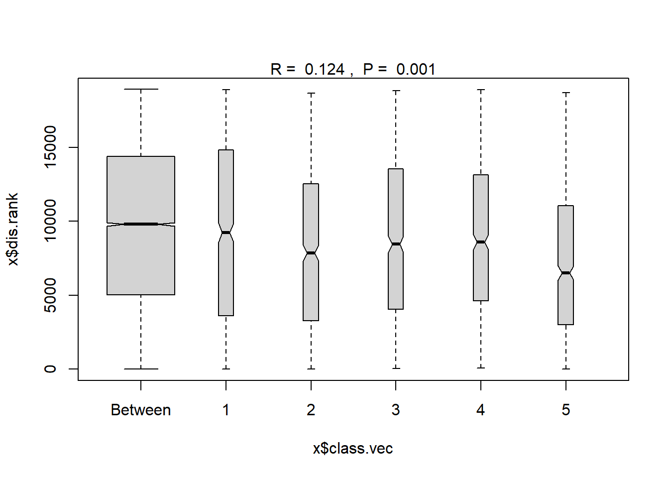
Region grouped
#region
ano_region_groups<- anosim(trawl_dist, trawl_data_arrange$REGION_NEW, permutations = 999)
ano_region_groups #regions are statistically different communities
##
## Call:
## anosim(x = trawl_dist, grouping = trawl_data_arrange$REGION_NEW, permutations = 999)
## Dissimilarity: bray
##
## ANOSIM statistic R: 0.06562
## Significance: 0.001
##
## Permutation: free
## Number of permutations: 999summary(ano_region_groups)##
## Call:
## anosim(x = trawl_dist, grouping = trawl_data_arrange$REGION_NEW, permutations = 999)
## Dissimilarity: bray
##
## ANOSIM statistic R: 0.06562
## Significance: 0.001
##
## Permutation: free
## Number of permutations: 999
##
## Upper quantiles of permutations (null model):
## 90% 95% 97.5% 99%
## 0.0198 0.0249 0.0308 0.0385
##
## Dissimilarity ranks between and within classes:
## 0% 25% 50% 75% 100% N
## Between 1 5017.5 9769.5 14357.5 18912 12168
## East of Penobscot Bay 3 4619.5 9134.0 13609.5 18915 3003
## Penobscot Bay 25 4040.0 8449.0 13533.0 18819 741
## West of Penobscot Bay 7 3949.5 8728.0 14093.0 18891 3003plot(ano_region_groups) #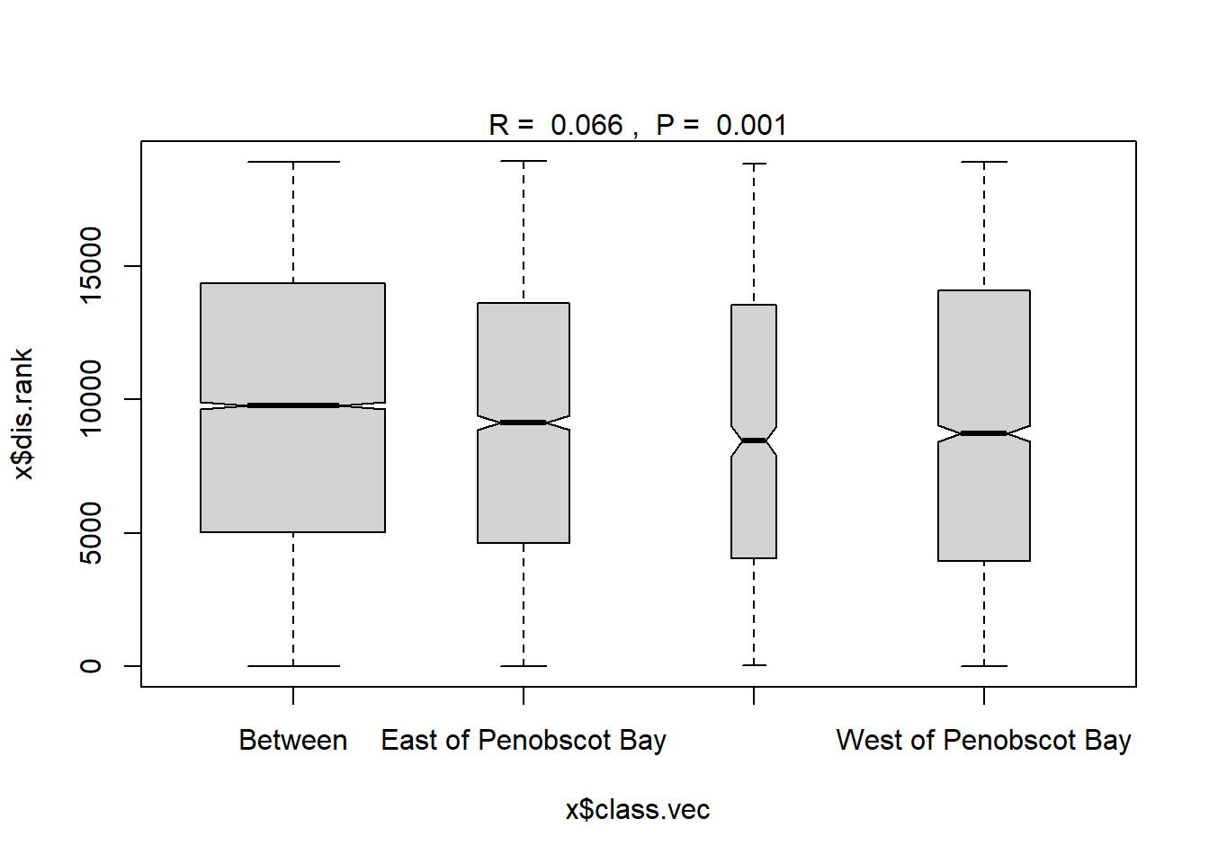
Year
#Time
ano_year<- anosim(trawl_dist, trawl_data_arrange$Year, permutations = 999)
ano_year #years are statistically different communities
##
## Call:
## anosim(x = trawl_dist, grouping = trawl_data_arrange$Year, permutations = 999)
## Dissimilarity: bray
##
## ANOSIM statistic R: 0.1498
## Significance: 0.001
##
## Permutation: free
## Number of permutations: 999summary(ano_year)##
## Call:
## anosim(x = trawl_dist, grouping = trawl_data_arrange$Year, permutations = 999)
## Dissimilarity: bray
##
## ANOSIM statistic R: 0.1498
## Significance: 0.001
##
## Permutation: free
## Number of permutations: 999
##
## Upper quantiles of permutations (null model):
## 90% 95% 97.5% 99%
## 0.0221 0.0291 0.0342 0.0380
##
## Dissimilarity ranks between and within classes:
## 0% 25% 50% 75% 100% N
## Between 1 4824.25 9554.5 14225.75 18915 18050
## 2000 373 5766.75 8332.5 11992.50 15706 10
## 2001 115 9203.00 14601.0 17569.00 18883 45
## 2002 291 6813.00 9501.0 13992.00 17835 45
## 2003 455 6975.00 10499.0 15855.00 17844 45
## 2004 103 8783.00 15421.0 18136.00 18898 45
## 2005 117 3297.00 7212.0 13687.00 18872 45
## 2006 293 5081.00 10098.0 13723.00 17705 45
## 2007 169 7647.00 12260.0 16295.00 18710 45
## 2008 365 4906.00 10248.0 15057.00 18497 45
## 2009 507 3430.00 6391.0 9482.00 16194 45
## 2010 221 2241.00 6186.0 9946.00 15162 45
## 2011 106 7826.00 11317.0 13950.00 17897 45
## 2012 177 1490.00 2412.0 5009.00 8908 45
## 2013 30 645.00 2514.0 4554.00 9911 45
## 2014 69 1666.00 4434.0 8999.00 16368 45
## 2015 116 4007.00 7956.0 10500.00 17186 45
## 2016 250 1740.00 4186.0 7165.00 13218 45
## 2017 215 1178.00 3156.0 6229.00 11872 45
## 2018 33 3676.00 8425.0 14101.00 17419 45
## 2019 35 3091.00 5574.0 10645.00 15825 45plot(ano_year)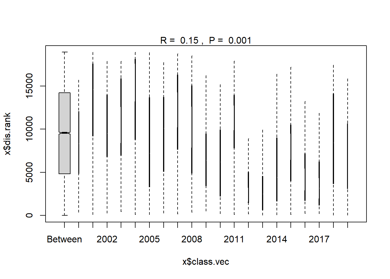
Year blocks
#Year blocks
ano_year_blocks<- anosim(trawl_dist, trawl_data_arrange$YEAR_GROUPS, permutations = 999)
ano_year_blocks #years are statistically different communities
##
## Call:
## anosim(x = trawl_dist, grouping = trawl_data_arrange$YEAR_GROUPS, permutations = 999)
## Dissimilarity: bray
##
## ANOSIM statistic R: 0.1776
## Significance: 0.001
##
## Permutation: free
## Number of permutations: 999summary(ano_year_blocks)##
## Call:
## anosim(x = trawl_dist, grouping = trawl_data_arrange$YEAR_GROUPS, permutations = 999)
## Dissimilarity: bray
##
## ANOSIM statistic R: 0.1776
## Significance: 0.001
##
## Permutation: free
## Number of permutations: 999
##
## Upper quantiles of permutations (null model):
## 90% 95% 97.5% 99%
## 0.00982 0.01438 0.01701 0.02196
##
## Dissimilarity ranks between and within classes:
## 0% 25% 50% 75% 100% N
## Between 1 5334.25 10060.5 14534.75 18915 14250
## 2000-2004 36 6576.75 12147.5 16277.50 18913 990
## 2005-2009 5 4347.00 8750.0 13859.00 18872 1225
## 2010-2014 28 2526.00 5616.0 9946.00 18144 1225
## 2015-2019 2 2430.00 5496.0 10153.00 18264 1225plot(ano_year_blocks)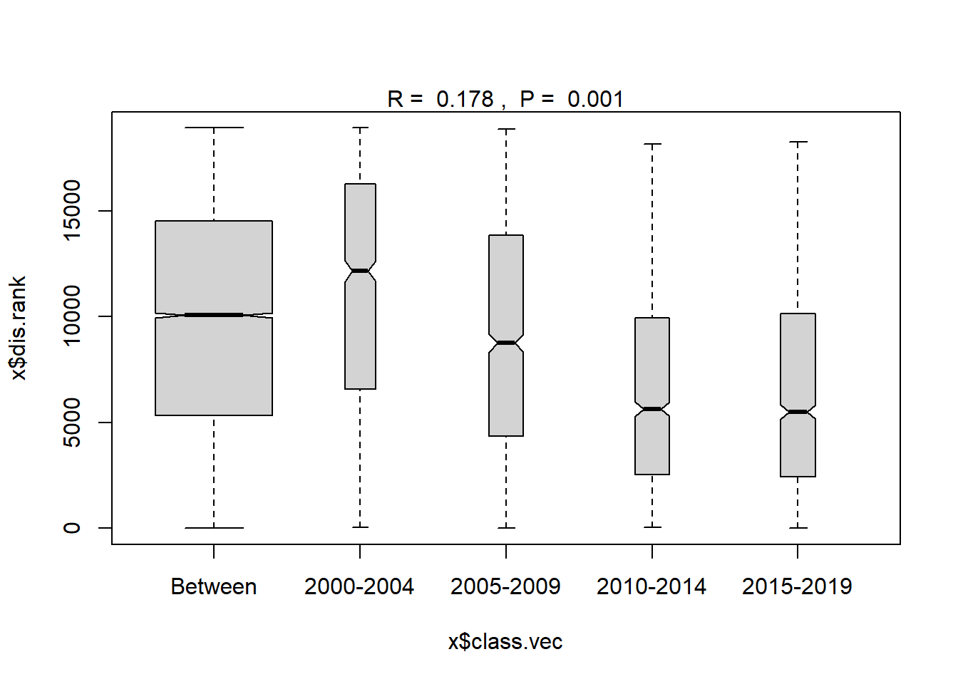
Analysis of variance (Adonis)
- Permanova
- tests whether there is a difference between means of groups
- works by calculating the sum of squares from the centroid of the group
Region
adonis<-adonis2(trawl_dist~Region, data=ME_group_data, by="terms", permutations = 9999)
adonis
## Permutation test for adonis under reduced model
## Terms added sequentially (first to last)
## Permutation: free
## Number of permutations: 9999
##
## adonis2(formula = trawl_dist ~ Region, data = ME_group_data, permutations = 9999, by = "terms")
## Df SumOfSqs R2 F Pr(>F)
## Region 1 1.0585 0.06221 12.803 1e-04 ***
## Residual 193 15.9564 0.93779
## Total 194 17.0148 1.00000
## ---
## Signif. codes: 0 '***' 0.001 '**' 0.01 '*' 0.05 '.' 0.1 ' ' 1summary(adonis)## Df SumOfSqs R2 F
## Min. : 1.0 Min. : 1.058 Min. :0.06221 Min. :12.8
## 1st Qu.: 97.0 1st Qu.: 8.507 1st Qu.:0.50000 1st Qu.:12.8
## Median :193.0 Median :15.956 Median :0.93779 Median :12.8
## Mean :129.3 Mean :11.343 Mean :0.66667 Mean :12.8
## 3rd Qu.:193.5 3rd Qu.:16.486 3rd Qu.:0.96890 3rd Qu.:12.8
## Max. :194.0 Max. :17.015 Max. :1.00000 Max. :12.8
## NA's :2
## Pr(>F)
## Min. :1e-04
## 1st Qu.:1e-04
## Median :1e-04
## Mean :1e-04
## 3rd Qu.:1e-04
## Max. :1e-04
## NA's :2Year
adonis<-adonis2(trawl_dist~Year, data=ME_group_data, by="terms", permutations = 9999)
adonis
## Permutation test for adonis under reduced model
## Terms added sequentially (first to last)
## Permutation: free
## Number of permutations: 9999
##
## adonis2(formula = trawl_dist ~ Year, data = ME_group_data, permutations = 9999, by = "terms")
## Df SumOfSqs R2 F Pr(>F)
## Year 1 1.682 0.09885 21.172 1e-04 ***
## Residual 193 15.333 0.90115
## Total 194 17.015 1.00000
## ---
## Signif. codes: 0 '***' 0.001 '**' 0.01 '*' 0.05 '.' 0.1 ' ' 1summary(adonis)## Df SumOfSqs R2 F
## Min. : 1.0 Min. : 1.682 Min. :0.09885 Min. :21.17
## 1st Qu.: 97.0 1st Qu.: 8.507 1st Qu.:0.50000 1st Qu.:21.17
## Median :193.0 Median :15.333 Median :0.90115 Median :21.17
## Mean :129.3 Mean :11.343 Mean :0.66667 Mean :21.17
## 3rd Qu.:193.5 3rd Qu.:16.174 3rd Qu.:0.95057 3rd Qu.:21.17
## Max. :194.0 Max. :17.015 Max. :1.00000 Max. :21.17
## NA's :2
## Pr(>F)
## Min. :1e-04
## 1st Qu.:1e-04
## Median :1e-04
## Mean :1e-04
## 3rd Qu.:1e-04
## Max. :1e-04
## NA's :2Region and Year
adonis<-adonis2(trawl_dist~Region*Year, data=ME_group_data, by="terms", permutations = 9999)
adonis
## Permutation test for adonis under reduced model
## Terms added sequentially (first to last)
## Permutation: free
## Number of permutations: 9999
##
## adonis2(formula = trawl_dist ~ Region * Year, data = ME_group_data, permutations = 9999, by = "terms")
## Df SumOfSqs R2 F Pr(>F)
## Region 1 1.0585 0.06221 14.5943 1e-04 ***
## Year 1 1.6820 0.09885 23.1915 1e-04 ***
## Region:Year 1 0.4218 0.02479 5.8157 4e-04 ***
## Residual 191 13.8526 0.81415
## Total 194 17.0148 1.00000
## ---
## Signif. codes: 0 '***' 0.001 '**' 0.01 '*' 0.05 '.' 0.1 ' ' 1summary(adonis)## Df SumOfSqs R2 F
## Min. : 1.0 Min. : 0.4218 Min. :0.02479 Min. : 5.816
## 1st Qu.: 1.0 1st Qu.: 1.0585 1st Qu.:0.06221 1st Qu.:10.205
## Median : 1.0 Median : 1.6820 Median :0.09885 Median :14.594
## Mean : 77.6 Mean : 6.8059 Mean :0.40000 Mean :14.534
## 3rd Qu.:191.0 3rd Qu.:13.8526 3rd Qu.:0.81415 3rd Qu.:18.893
## Max. :194.0 Max. :17.0148 Max. :1.00000 Max. :23.191
## NA's :2
## Pr(>F)
## Min. :0.00010
## 1st Qu.:0.00010
## Median :0.00010
## Mean :0.00020
## 3rd Qu.:0.00025
## Max. :0.00040
## NA's :2year block
#with year blocks
adonis<-adonis2(trawl_dist~YEAR_GROUPS, data=ME_group_data, by="terms", permutations = 9999)
adonis
## Permutation test for adonis under reduced model
## Terms added sequentially (first to last)
## Permutation: free
## Number of permutations: 9999
##
## adonis2(formula = trawl_dist ~ YEAR_GROUPS, data = ME_group_data, permutations = 9999, by = "terms")
## Df SumOfSqs R2 F Pr(>F)
## YEAR_GROUPS 3 2.4691 0.14511 10.807 1e-04 ***
## Residual 191 14.5458 0.85489
## Total 194 17.0148 1.00000
## ---
## Signif. codes: 0 '***' 0.001 '**' 0.01 '*' 0.05 '.' 0.1 ' ' 1summary(adonis)## Df SumOfSqs R2 F
## Min. : 3.0 Min. : 2.469 Min. :0.1451 Min. :10.81
## 1st Qu.: 97.0 1st Qu.: 8.507 1st Qu.:0.5000 1st Qu.:10.81
## Median :191.0 Median :14.546 Median :0.8549 Median :10.81
## Mean :129.3 Mean :11.343 Mean :0.6667 Mean :10.81
## 3rd Qu.:192.5 3rd Qu.:15.780 3rd Qu.:0.9274 3rd Qu.:10.81
## Max. :194.0 Max. :17.015 Max. :1.0000 Max. :10.81
## NA's :2
## Pr(>F)
## Min. :1e-04
## 1st Qu.:1e-04
## Median :1e-04
## Mean :1e-04
## 3rd Qu.:1e-04
## Max. :1e-04
## NA's :2Region and year block
#with year blocks
adonis<-adonis2(trawl_dist~Region*YEAR_GROUPS, data=ME_group_data, by="terms", permutations = 9999)
adonis
## Permutation test for adonis under reduced model
## Terms added sequentially (first to last)
## Permutation: free
## Number of permutations: 9999
##
## adonis2(formula = trawl_dist ~ Region * YEAR_GROUPS, data = ME_group_data, permutations = 9999, by = "terms")
## Df SumOfSqs R2 F Pr(>F)
## Region 1 1.0585 0.06221 15.3325 0.0001 ***
## YEAR_GROUPS 3 2.4691 0.14511 11.9218 0.0001 ***
## Region:YEAR_GROUPS 3 0.5778 0.03396 2.7898 0.0013 **
## Residual 187 12.9095 0.75872
## Total 194 17.0148 1.00000
## ---
## Signif. codes: 0 '***' 0.001 '**' 0.01 '*' 0.05 '.' 0.1 ' ' 1summary(adonis)## Df SumOfSqs R2 F
## Min. : 1.0 Min. : 0.5778 Min. :0.03396 Min. : 2.790
## 1st Qu.: 3.0 1st Qu.: 1.0585 1st Qu.:0.06221 1st Qu.: 7.356
## Median : 3.0 Median : 2.4691 Median :0.14511 Median :11.922
## Mean : 77.6 Mean : 6.8059 Mean :0.40000 Mean :10.015
## 3rd Qu.:187.0 3rd Qu.:12.9095 3rd Qu.:0.75872 3rd Qu.:13.627
## Max. :194.0 Max. :17.0148 Max. :1.00000 Max. :15.332
## NA's :2
## Pr(>F)
## Min. :0.0001
## 1st Qu.:0.0001
## Median :0.0001
## Mean :0.0005
## 3rd Qu.:0.0007
## Max. :0.0013
## NA's :2Region groups
#with year blocks
adonis<-adonis2(trawl_dist~REGION_NEW, data=ME_group_data, by="terms", permutations = 9999)
adonis
## Permutation test for adonis under reduced model
## Terms added sequentially (first to last)
## Permutation: free
## Number of permutations: 9999
##
## adonis2(formula = trawl_dist ~ REGION_NEW, data = ME_group_data, permutations = 9999, by = "terms")
## Df SumOfSqs R2 F Pr(>F)
## REGION_NEW 2 1.0531 0.06189 6.3335 1e-04 ***
## Residual 192 15.9618 0.93811
## Total 194 17.0148 1.00000
## ---
## Signif. codes: 0 '***' 0.001 '**' 0.01 '*' 0.05 '.' 0.1 ' ' 1summary(adonis)## Df SumOfSqs R2 F
## Min. : 2.0 Min. : 1.053 Min. :0.06189 Min. :6.333
## 1st Qu.: 97.0 1st Qu.: 8.507 1st Qu.:0.50000 1st Qu.:6.333
## Median :192.0 Median :15.962 Median :0.93811 Median :6.333
## Mean :129.3 Mean :11.343 Mean :0.66667 Mean :6.333
## 3rd Qu.:193.0 3rd Qu.:16.488 3rd Qu.:0.96905 3rd Qu.:6.333
## Max. :194.0 Max. :17.015 Max. :1.00000 Max. :6.333
## NA's :2
## Pr(>F)
## Min. :1e-04
## 1st Qu.:1e-04
## Median :1e-04
## Mean :1e-04
## 3rd Qu.:1e-04
## Max. :1e-04
## NA's :2Region groups and year block
#with year blocks
adonis<-adonis2(trawl_dist~REGION_NEW*YEAR_GROUPS, data=ME_group_data, by="terms", permutations = 9999)
adonis
## Permutation test for adonis under reduced model
## Terms added sequentially (first to last)
## Permutation: free
## Number of permutations: 9999
##
## adonis2(formula = trawl_dist ~ REGION_NEW * YEAR_GROUPS, data = ME_group_data, permutations = 9999, by = "terms")
## Df SumOfSqs R2 F Pr(>F)
## REGION_NEW 2 1.0531 0.06189 7.5651 0.0001 ***
## YEAR_GROUPS 3 2.4691 0.14511 11.8249 0.0001 ***
## REGION_NEW:YEAR_GROUPS 6 0.7559 0.04443 1.8101 0.0154 *
## Residual 183 12.7368 0.74857
## Total 194 17.0148 1.00000
## ---
## Signif. codes: 0 '***' 0.001 '**' 0.01 '*' 0.05 '.' 0.1 ' ' 1summary(adonis)## Df SumOfSqs R2 F
## Min. : 2.0 Min. : 0.7559 Min. :0.04443 Min. : 1.810
## 1st Qu.: 3.0 1st Qu.: 1.0531 1st Qu.:0.06189 1st Qu.: 4.688
## Median : 6.0 Median : 2.4691 Median :0.14511 Median : 7.565
## Mean : 77.6 Mean : 6.8059 Mean :0.40000 Mean : 7.067
## 3rd Qu.:183.0 3rd Qu.:12.7368 3rd Qu.:0.74857 3rd Qu.: 9.695
## Max. :194.0 Max. :17.0148 Max. :1.00000 Max. :11.825
## NA's :2
## Pr(>F)
## Min. :0.00010
## 1st Qu.:0.00010
## Median :0.00010
## Mean :0.00520
## 3rd Qu.:0.00775
## Max. :0.01540
## NA's :2Pairwise
- Vegan does not have a function for this, but I found a wrapper that seems frequently used on github
- select groups to test, one pair at a time
- Adjust p-values for multiple tests
Region
#pair-wise test to see what is different
pair<-pairwise.adonis2(trawl_dist~Region, data=ME_group_data, by="terms", permutations = 9999)
summary(pair)
## Length Class Mode
## parent_call 1 -none- character
## 1_vs_2 6 anova list
## 1_vs_3 6 anova list
## 1_vs_4 6 anova list
## 1_vs_5 6 anova list
## 2_vs_3 6 anova list
## 2_vs_4 6 anova list
## 2_vs_5 6 anova list
## 3_vs_4 6 anova list
## 3_vs_5 6 anova list
## 4_vs_5 6 anova listpair ## $parent_call
## [1] "trawl_dist ~ Region , strata = Null"
##
## $`1_vs_2`
## Permutation: free
## Number of permutations: 9999
##
## Terms added sequentially (first to last)
##
## Df SumsOfSqs MeanSqs F.Model R2 Pr(>F)
## Region 1 0.2871 0.287090 3.5682 0.04484 0.021 *
## Residuals 76 6.1148 0.080457 0.95516
## Total 77 6.4018 1.00000
## ---
## Signif. codes: 0 '***' 0.001 '**' 0.01 '*' 0.05 '.' 0.1 ' ' 1
##
## $`1_vs_3`
## Permutation: free
## Number of permutations: 9999
##
## Terms added sequentially (first to last)
##
## Df SumsOfSqs MeanSqs F.Model R2 Pr(>F)
## Region 1 0.4635 0.46349 5.4721 0.06716 0.0017 **
## Residuals 76 6.4373 0.08470 0.93284
## Total 77 6.9008 1.00000
## ---
## Signif. codes: 0 '***' 0.001 '**' 0.01 '*' 0.05 '.' 0.1 ' ' 1
##
## $`1_vs_4`
## Permutation: free
## Number of permutations: 9999
##
## Terms added sequentially (first to last)
##
## Df SumsOfSqs MeanSqs F.Model R2 Pr(>F)
## Region 1 0.5648 0.56479 6.6633 0.08061 4e-04 ***
## Residuals 76 6.4419 0.08476 0.91939
## Total 77 7.0067 1.00000
## ---
## Signif. codes: 0 '***' 0.001 '**' 0.01 '*' 0.05 '.' 0.1 ' ' 1
##
## $`1_vs_5`
## Permutation: free
## Number of permutations: 9999
##
## Terms added sequentially (first to last)
##
## Df SumsOfSqs MeanSqs F.Model R2 Pr(>F)
## Region 1 1.0276 1.02765 13.532 0.15114 1e-04 ***
## Residuals 76 5.7716 0.07594 0.84886
## Total 77 6.7992 1.00000
## ---
## Signif. codes: 0 '***' 0.001 '**' 0.01 '*' 0.05 '.' 0.1 ' ' 1
##
## $`2_vs_3`
## Permutation: free
## Number of permutations: 9999
##
## Terms added sequentially (first to last)
##
## Df SumsOfSqs MeanSqs F.Model R2 Pr(>F)
## Region 1 0.1174 0.117432 1.5268 0.01969 0.1906
## Residuals 76 5.8455 0.076914 0.98031
## Total 77 5.9629 1.00000
##
## $`2_vs_4`
## Permutation: free
## Number of permutations: 9999
##
## Terms added sequentially (first to last)
##
## Df SumsOfSqs MeanSqs F.Model R2 Pr(>F)
## Region 1 0.2133 0.213305 2.7711 0.03518 0.0341 *
## Residuals 76 5.8501 0.076976 0.96482
## Total 77 6.0634 1.00000
## ---
## Signif. codes: 0 '***' 0.001 '**' 0.01 '*' 0.05 '.' 0.1 ' ' 1
##
## $`2_vs_5`
## Permutation: free
## Number of permutations: 9999
##
## Terms added sequentially (first to last)
##
## Df SumsOfSqs MeanSqs F.Model R2 Pr(>F)
## Region 1 1.1755 1.17549 17.247 0.18496 1e-04 ***
## Residuals 76 5.1798 0.06816 0.81504
## Total 77 6.3553 1.00000
## ---
## Signif. codes: 0 '***' 0.001 '**' 0.01 '*' 0.05 '.' 0.1 ' ' 1
##
## $`3_vs_4`
## Permutation: free
## Number of permutations: 9999
##
## Terms added sequentially (first to last)
##
## Df SumsOfSqs MeanSqs F.Model R2 Pr(>F)
## Region 1 0.0864 0.086413 1.0639 0.01381 0.3688
## Residuals 76 6.1727 0.081219 0.98619
## Total 77 6.2591 1.00000
##
## $`3_vs_5`
## Permutation: free
## Number of permutations: 9999
##
## Terms added sequentially (first to last)
##
## Df SumsOfSqs MeanSqs F.Model R2 Pr(>F)
## Region 1 0.8681 0.86814 11.991 0.13628 1e-04 ***
## Residuals 76 5.5023 0.07240 0.86372
## Total 77 6.3705 1.00000
## ---
## Signif. codes: 0 '***' 0.001 '**' 0.01 '*' 0.05 '.' 0.1 ' ' 1
##
## $`4_vs_5`
## Permutation: free
## Number of permutations: 9999
##
## Terms added sequentially (first to last)
##
## Df SumsOfSqs MeanSqs F.Model R2 Pr(>F)
## Region 1 0.9690 0.96895 13.372 0.14962 1e-04 ***
## Residuals 76 5.5070 0.07246 0.85038
## Total 77 6.4759 1.00000
## ---
## Signif. codes: 0 '***' 0.001 '**' 0.01 '*' 0.05 '.' 0.1 ' ' 1
##
## attr(,"class")
## [1] "pwadstrata" "list"Region groups
#pair-wise test to see what is different
pair<-pairwise.adonis2(trawl_dist~REGION_NEW, data=ME_group_data, by="terms", permutations = 9999)
summary(pair)
## Length Class Mode
## parent_call 1 -none- character
## West of Penobscot Bay_vs_Penobscot Bay 6 anova list
## West of Penobscot Bay_vs_East of Penobscot Bay 6 anova list
## Penobscot Bay_vs_East of Penobscot Bay 6 anova listpair ## $parent_call
## [1] "trawl_dist ~ REGION_NEW , strata = Null"
##
## $`West of Penobscot Bay_vs_Penobscot Bay`
## Permutation: free
## Number of permutations: 9999
##
## Terms added sequentially (first to last)
##
## Df SumsOfSqs MeanSqs F.Model R2 Pr(>F)
## REGION_NEW 1 0.2916 0.291584 3.535 0.02982 0.0132 *
## Residuals 115 9.4858 0.082486 0.97018
## Total 116 9.7774 1.00000
## ---
## Signif. codes: 0 '***' 0.001 '**' 0.01 '*' 0.05 '.' 0.1 ' ' 1
##
## $`West of Penobscot Bay_vs_East of Penobscot Bay`
## Permutation: free
## Number of permutations: 9999
##
## Terms added sequentially (first to last)
##
## Df SumsOfSqs MeanSqs F.Model R2 Pr(>F)
## REGION_NEW 1 0.8626 0.86260 10.315 0.06278 1e-04 ***
## Residuals 154 12.8778 0.08362 0.93722
## Total 155 13.7404 1.00000
## ---
## Signif. codes: 0 '***' 0.001 '**' 0.01 '*' 0.05 '.' 0.1 ' ' 1
##
## $`Penobscot Bay_vs_East of Penobscot Bay`
## Permutation: free
## Number of permutations: 9999
##
## Terms added sequentially (first to last)
##
## Df SumsOfSqs MeanSqs F.Model R2 Pr(>F)
## REGION_NEW 1 0.3134 0.31338 3.7698 0.03174 0.0083 **
## Residuals 115 9.5599 0.08313 0.96826
## Total 116 9.8733 1.00000
## ---
## Signif. codes: 0 '***' 0.001 '**' 0.01 '*' 0.05 '.' 0.1 ' ' 1
##
## attr(,"class")
## [1] "pwadstrata" "list"Year blocks
#pair-wise test to see what is different for year blocks
pair<-pairwise.adonis2(trawl_dist~YEAR_GROUPS, data=ME_group_data, by="terms", permutations = 9999)
summary(pair)
## Length Class Mode
## parent_call 1 -none- character
## 2000-2004_vs_2005-2009 6 anova list
## 2000-2004_vs_2010-2014 6 anova list
## 2000-2004_vs_2015-2019 6 anova list
## 2005-2009_vs_2010-2014 6 anova list
## 2005-2009_vs_2015-2019 6 anova list
## 2010-2014_vs_2015-2019 6 anova listpair## $parent_call
## [1] "trawl_dist ~ YEAR_GROUPS , strata = Null"
##
## $`2000-2004_vs_2005-2009`
## Permutation: free
## Number of permutations: 9999
##
## Terms added sequentially (first to last)
##
## Df SumsOfSqs MeanSqs F.Model R2 Pr(>F)
## YEAR_GROUPS 1 0.4868 0.48684 4.9616 0.05065 0.0023 **
## Residuals 93 9.1253 0.09812 0.94935
## Total 94 9.6122 1.00000
## ---
## Signif. codes: 0 '***' 0.001 '**' 0.01 '*' 0.05 '.' 0.1 ' ' 1
##
## $`2000-2004_vs_2010-2014`
## Permutation: free
## Number of permutations: 9999
##
## Terms added sequentially (first to last)
##
## Df SumsOfSqs MeanSqs F.Model R2 Pr(>F)
## YEAR_GROUPS 1 0.6501 0.65005 7.9359 0.07862 1e-04 ***
## Residuals 93 7.6179 0.08191 0.92138
## Total 94 8.2679 1.00000
## ---
## Signif. codes: 0 '***' 0.001 '**' 0.01 '*' 0.05 '.' 0.1 ' ' 1
##
## $`2000-2004_vs_2015-2019`
## Permutation: free
## Number of permutations: 9999
##
## Terms added sequentially (first to last)
##
## Df SumsOfSqs MeanSqs F.Model R2 Pr(>F)
## YEAR_GROUPS 1 1.2574 1.25744 15.327 0.14149 1e-04 ***
## Residuals 93 7.6300 0.08204 0.85851
## Total 94 8.8874 1.00000
## ---
## Signif. codes: 0 '***' 0.001 '**' 0.01 '*' 0.05 '.' 0.1 ' ' 1
##
## $`2005-2009_vs_2010-2014`
## Permutation: free
## Number of permutations: 9999
##
## Terms added sequentially (first to last)
##
## Df SumsOfSqs MeanSqs F.Model R2 Pr(>F)
## YEAR_GROUPS 1 0.6698 0.66983 9.4918 0.0883 1e-04 ***
## Residuals 98 6.9158 0.07057 0.9117
## Total 99 7.5856 1.0000
## ---
## Signif. codes: 0 '***' 0.001 '**' 0.01 '*' 0.05 '.' 0.1 ' ' 1
##
## $`2005-2009_vs_2015-2019`
## Permutation: free
## Number of permutations: 9999
##
## Terms added sequentially (first to last)
##
## Df SumsOfSqs MeanSqs F.Model R2 Pr(>F)
## YEAR_GROUPS 1 1.5860 1.58600 22.435 0.18628 1e-04 ***
## Residuals 98 6.9279 0.07069 0.81372
## Total 99 8.5139 1.00000
## ---
## Signif. codes: 0 '***' 0.001 '**' 0.01 '*' 0.05 '.' 0.1 ' ' 1
##
## $`2010-2014_vs_2015-2019`
## Permutation: free
## Number of permutations: 9999
##
## Terms added sequentially (first to last)
##
## Df SumsOfSqs MeanSqs F.Model R2 Pr(>F)
## YEAR_GROUPS 1 0.2842 0.284204 5.1383 0.04982 0.001 ***
## Residuals 98 5.4205 0.055311 0.95018
## Total 99 5.7047 1.00000
## ---
## Signif. codes: 0 '***' 0.001 '**' 0.01 '*' 0.05 '.' 0.1 ' ' 1
##
## attr(,"class")
## [1] "pwadstrata" "list"Dispersion
- anosim very sensitive to heterogeneity (Anderson and Walsh 2013)
- Could get false significant results from differences in variance instead of mean
- adonis is less affected by heterogeneity for balanced designs
- PRIMER can deal with dispersion issues, but vegan does not yet
- tests null hypothesis that there is no difference in dispersion between groups
- p-value <0.05 means difference is significant
Region
#betadisper test homogeneity of dispersion among groups
#Region
bd<-betadisper(trawl_dist,ME_group_data$Region)
bd
##
## Homogeneity of multivariate dispersions
##
## Call: betadisper(d = trawl_dist, group = ME_group_data$Region)
##
## No. of Positive Eigenvalues: 61
## No. of Negative Eigenvalues: 133
##
## Average distance to median:
## 1 2 3 4 5
## 0.2756 0.2524 0.2629 0.2638 0.2320
##
## Eigenvalues for PCoA axes:
## (Showing 8 of 194 eigenvalues)
## PCoA1 PCoA2 PCoA3 PCoA4 PCoA5 PCoA6 PCoA7 PCoA8
## 6.8676 3.9273 2.9139 1.5004 1.1849 0.9763 0.6387 0.6009anova(bd) ## Analysis of Variance Table
##
## Response: Distances
## Df Sum Sq Mean Sq F value Pr(>F)
## Groups 4 0.04183 0.010458 1.042 0.3868
## Residuals 190 1.90702 0.010037#test based on permutations
permutest(bd)##
## Permutation test for homogeneity of multivariate dispersions
## Permutation: free
## Number of permutations: 999
##
## Response: Distances
## Df Sum Sq Mean Sq F N.Perm Pr(>F)
## Groups 4 0.04183 0.010458 1.042 999 0.386
## Residuals 190 1.90702 0.010037plot(bd, hull=FALSE, ellipse = TRUE) 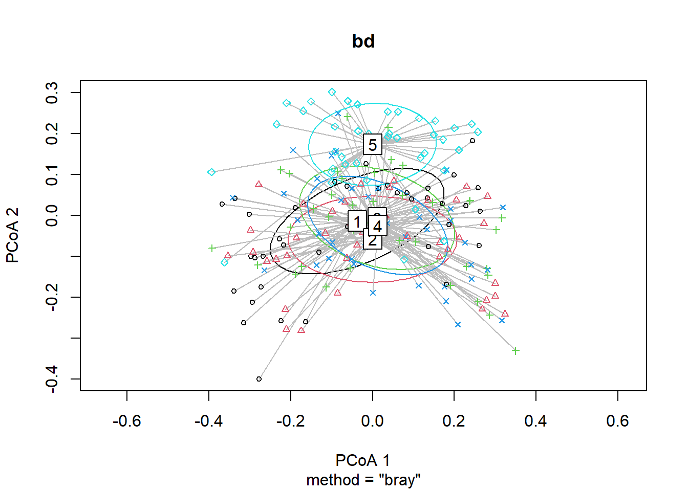
boxplot(bd)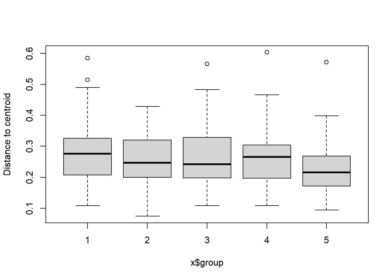
Region group
#Region
bd<-betadisper(trawl_dist,ME_group_data$REGION_NEW)
bd
##
## Homogeneity of multivariate dispersions
##
## Call: betadisper(d = trawl_dist, group = ME_group_data$REGION_NEW)
##
## No. of Positive Eigenvalues: 61
## No. of Negative Eigenvalues: 133
##
## Average distance to median:
## East of Penobscot Bay Penobscot Bay West of Penobscot Bay
## 0.2703 0.2629 0.2713
##
## Eigenvalues for PCoA axes:
## (Showing 8 of 194 eigenvalues)
## PCoA1 PCoA2 PCoA3 PCoA4 PCoA5 PCoA6 PCoA7 PCoA8
## 6.8676 3.9273 2.9139 1.5004 1.1849 0.9763 0.6387 0.6009anova(bd) ## Analysis of Variance Table
##
## Response: Distances
## Df Sum Sq Mean Sq F value Pr(>F)
## Groups 2 0.00195 0.0009725 0.0946 0.9098
## Residuals 192 1.97337 0.0102780#test based on permutations
permutest(bd)##
## Permutation test for homogeneity of multivariate dispersions
## Permutation: free
## Number of permutations: 999
##
## Response: Distances
## Df Sum Sq Mean Sq F N.Perm Pr(>F)
## Groups 2 0.00195 0.0009725 0.0946 999 0.905
## Residuals 192 1.97337 0.0102780plot(bd, hull=FALSE, ellipse = TRUE) 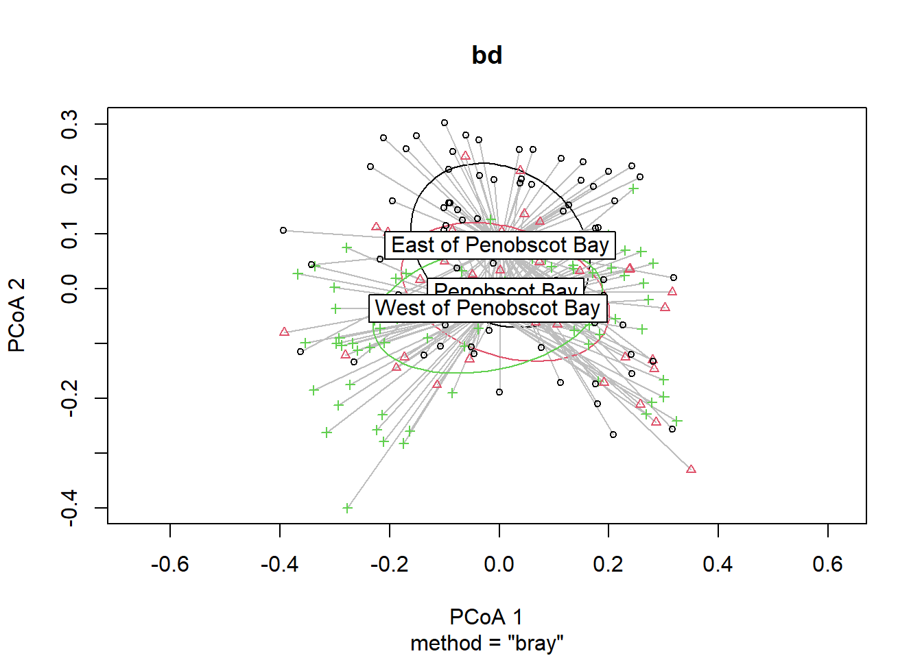
boxplot(bd)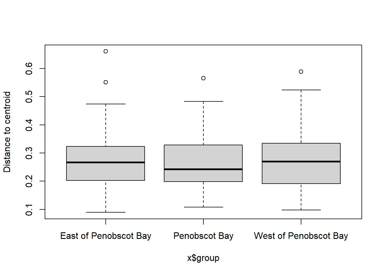
Year
#Year
bd<-betadisper(trawl_dist,ME_group_data$Year)
bd
##
## Homogeneity of multivariate dispersions
##
## Call: betadisper(d = trawl_dist, group = ME_group_data$Year)
##
## No. of Positive Eigenvalues: 61
## No. of Negative Eigenvalues: 133
##
## Average distance to median:
## 2000 2001 2002 2003 2004 2005 2006 2007 2008 2009 2010
## 0.2369 0.3367 0.2638 0.2921 0.3425 0.2455 0.2583 0.3055 0.2609 0.2183 0.2068
## 2011 2012 2013 2014 2015 2016 2017 2018 2019
## 0.2721 0.1533 0.1379 0.1856 0.2254 0.1825 0.1624 0.2536 0.2014
##
## Eigenvalues for PCoA axes:
## (Showing 8 of 194 eigenvalues)
## PCoA1 PCoA2 PCoA3 PCoA4 PCoA5 PCoA6 PCoA7 PCoA8
## 6.8676 3.9273 2.9139 1.5004 1.1849 0.9763 0.6387 0.6009anova(bd) ## Analysis of Variance Table
##
## Response: Distances
## Df Sum Sq Mean Sq F value Pr(>F)
## Groups 19 0.62783 0.033044 3.2075 2.545e-05 ***
## Residuals 175 1.80285 0.010302
## ---
## Signif. codes: 0 '***' 0.001 '**' 0.01 '*' 0.05 '.' 0.1 ' ' 1#test based on permutations
permutest(bd)##
## Permutation test for homogeneity of multivariate dispersions
## Permutation: free
## Number of permutations: 999
##
## Response: Distances
## Df Sum Sq Mean Sq F N.Perm Pr(>F)
## Groups 19 0.62783 0.033044 3.2075 999 0.001 ***
## Residuals 175 1.80285 0.010302
## ---
## Signif. codes: 0 '***' 0.001 '**' 0.01 '*' 0.05 '.' 0.1 ' ' 1plot(bd, hull=FALSE, ellipse = TRUE)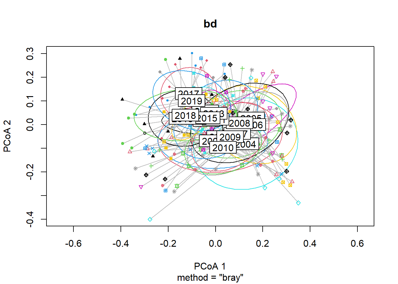
boxplot(bd)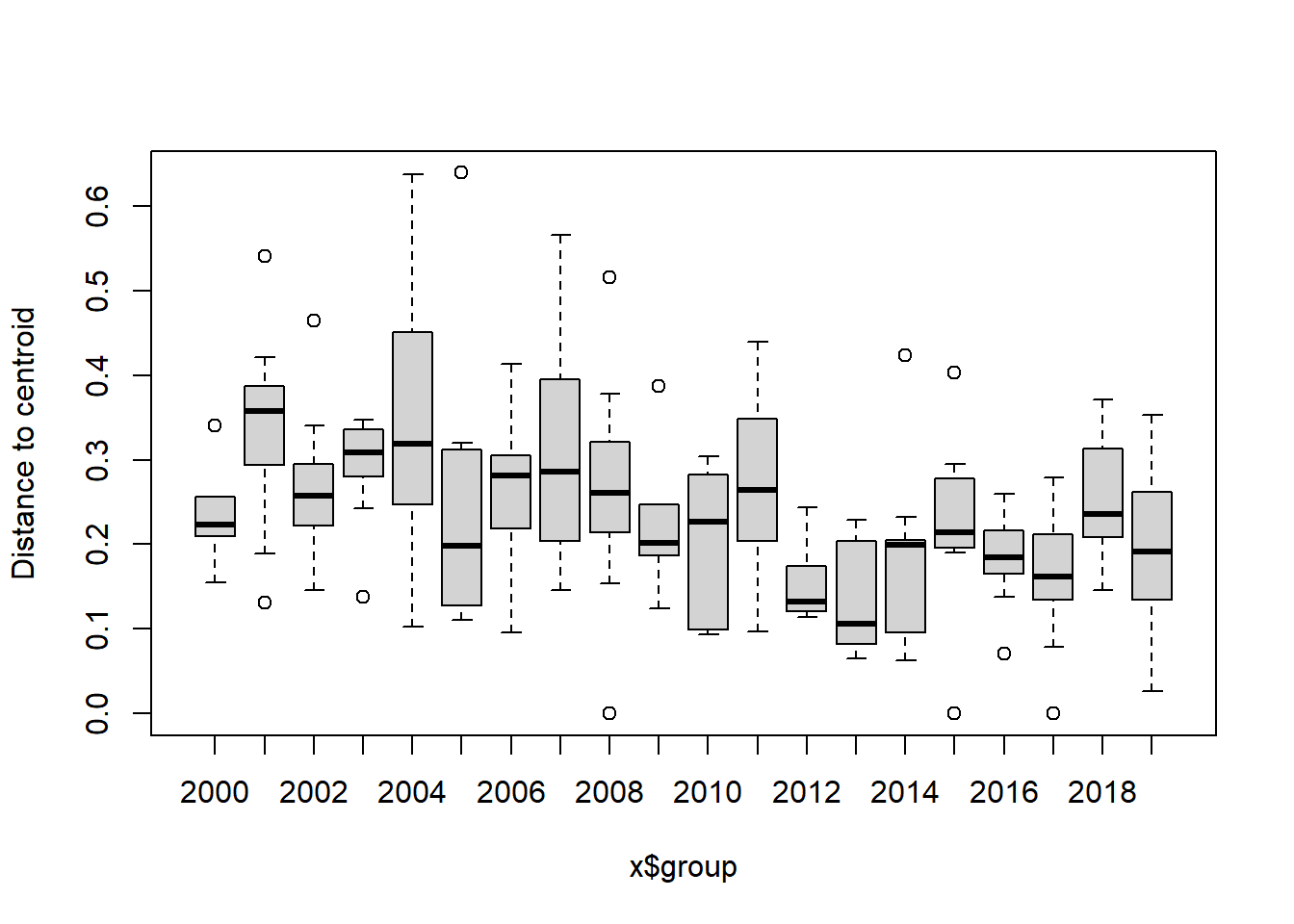
Year block
#Year blocks
bd<-betadisper(trawl_dist,ME_group_data$YEAR_GROUPS)
bd
##
## Homogeneity of multivariate dispersions
##
## Call: betadisper(d = trawl_dist, group = ME_group_data$YEAR_GROUPS)
##
## No. of Positive Eigenvalues: 61
## No. of Negative Eigenvalues: 133
##
## Average distance to median:
## 2000-2004 2005-2009 2010-2014 2015-2019
## 0.3146 0.2701 0.2153 0.2172
##
## Eigenvalues for PCoA axes:
## (Showing 8 of 194 eigenvalues)
## PCoA1 PCoA2 PCoA3 PCoA4 PCoA5 PCoA6 PCoA7 PCoA8
## 6.8676 3.9273 2.9139 1.5004 1.1849 0.9763 0.6387 0.6009anova(bd) ## Analysis of Variance Table
##
## Response: Distances
## Df Sum Sq Mean Sq F value Pr(>F)
## Groups 3 0.3205 0.106833 10.883 1.241e-06 ***
## Residuals 191 1.8749 0.009816
## ---
## Signif. codes: 0 '***' 0.001 '**' 0.01 '*' 0.05 '.' 0.1 ' ' 1#test based on permutations
permutest(bd)##
## Permutation test for homogeneity of multivariate dispersions
## Permutation: free
## Number of permutations: 999
##
## Response: Distances
## Df Sum Sq Mean Sq F N.Perm Pr(>F)
## Groups 3 0.3205 0.106833 10.883 999 0.001 ***
## Residuals 191 1.8749 0.009816
## ---
## Signif. codes: 0 '***' 0.001 '**' 0.01 '*' 0.05 '.' 0.1 ' ' 1plot(bd, hull=FALSE, ellipse = TRUE)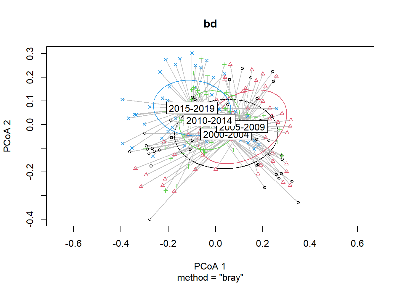
boxplot(bd)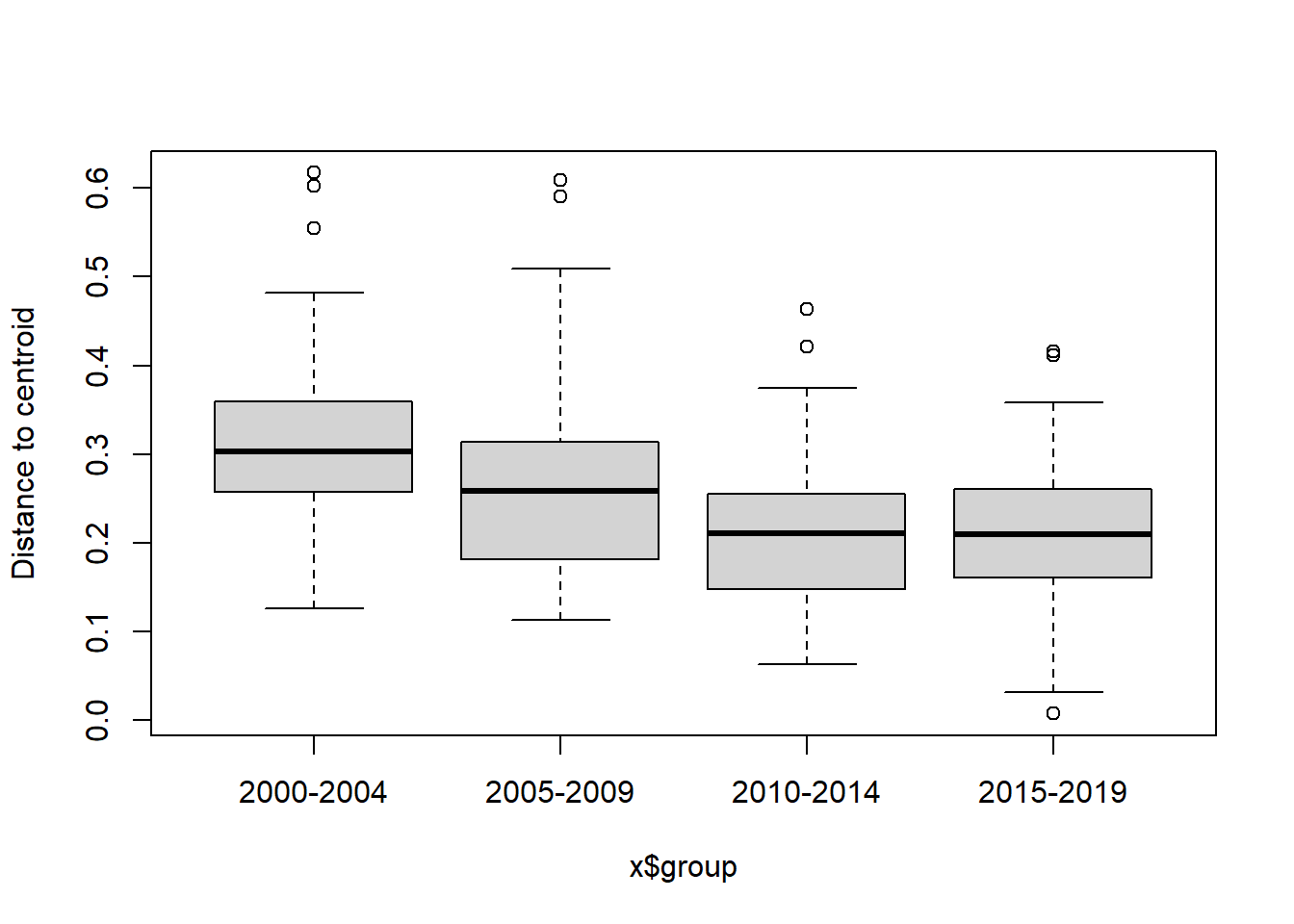
Indicator species analysis
- test if a species if found significantly more in one group compared to another
- all combinations of groups
Region
#see which species are found significantly more in each Region
inv_region<-multipatt(ME_NMDS_data, ME_group_data$Region, func = "r.g", control = how(nperm=999))
summary(inv_region)
##
## Multilevel pattern analysis
## ---------------------------
##
## Association function: r.g
## Significance level (alpha): 0.05
##
## Total number of species: 5
## Selected number of species: 4
## Number of species associated to 1 group: 2
## Number of species associated to 2 groups: 0
## Number of species associated to 3 groups: 1
## Number of species associated to 4 groups: 1
##
## List of species associated to each combination:
##
## Group 1 #sps. 1
## stat p.value
## piscivore 0.346 0.001 ***
##
## Group 4 #sps. 1
## stat p.value
## benthos 0.282 0.001 ***
##
## Group 2+3+4 #sps. 1
## stat p.value
## undefined 0.309 0.001 ***
##
## Group 1+2+3+4 #sps. 1
## stat p.value
## planktivore 0.381 0.001 ***
## ---
## Signif. codes: 0 '***' 0.001 '**' 0.01 '*' 0.05 '.' 0.1 ' ' 1Year block
#see which species are found significantly more in each Region
inv_year<-multipatt(ME_NMDS_data, ME_group_data$YEAR_GROUPS, func = "r.g", control = how(nperm=999))
summary(inv_year)##
## Multilevel pattern analysis
## ---------------------------
##
## Association function: r.g
## Significance level (alpha): 0.05
##
## Total number of species: 5
## Selected number of species: 2
## Number of species associated to 1 group: 0
## Number of species associated to 2 groups: 2
## Number of species associated to 3 groups: 0
##
## List of species associated to each combination:
##
## Group 2005-2009+2010-2014 #sps. 1
## stat p.value
## undefined 0.314 0.001 ***
##
## Group 2010-2014+2015-2019 #sps. 1
## stat p.value
## benthivore 0.514 0.001 ***
## ---
## Signif. codes: 0 '***' 0.001 '**' 0.01 '*' 0.05 '.' 0.1 ' ' 1Data- Abundance functional groups
- average across depth strata using the NOAA IEA technical document
- calculate dissimilarity matrix with Bray-Curtis distances
Analysis of similarity (Anosim)
- tests statistically whether there is a significant difference between two or more groups
- works by testing if distances between groups are greater than within groups
- significant values mean that there is a statistically significant difference in the communities between the groups
- R statistic closer to 1 is more dissimilar
Region
#region
ano_region<- anosim(trawl_dist, trawl_data_arrange$Region, permutations = 999)
ano_region #regions are statistically different communities ##
## Call:
## anosim(x = trawl_dist, grouping = trawl_data_arrange$Region, permutations = 999)
## Dissimilarity: bray
##
## ANOSIM statistic R: 0.175
## Significance: 0.001
##
## Permutation: free
## Number of permutations: 999summary(ano_region)##
## Call:
## anosim(x = trawl_dist, grouping = trawl_data_arrange$Region, permutations = 999)
## Dissimilarity: bray
##
## ANOSIM statistic R: 0.175
## Significance: 0.001
##
## Permutation: free
## Number of permutations: 999
##
## Upper quantiles of permutations (null model):
## 90% 95% 97.5% 99%
## 0.0123 0.0174 0.0226 0.0309
##
## Dissimilarity ranks between and within classes:
## 0% 25% 50% 75% 100% N
## Between 1 4876.25 9508.5 13973.25 18145 14590
## 1 4 3446.00 7647.0 11904.00 17887 741
## 2 15 2935.00 6728.0 11581.00 17675 741
## 3 10 2901.00 6546.5 10943.75 17683 666
## 4 17 3019.00 6891.5 11499.50 18077 666
## 5 39 5049.00 9206.0 13537.00 18031 741plot(ano_region) #regions don't look very different in plot though...confidence bands all overlap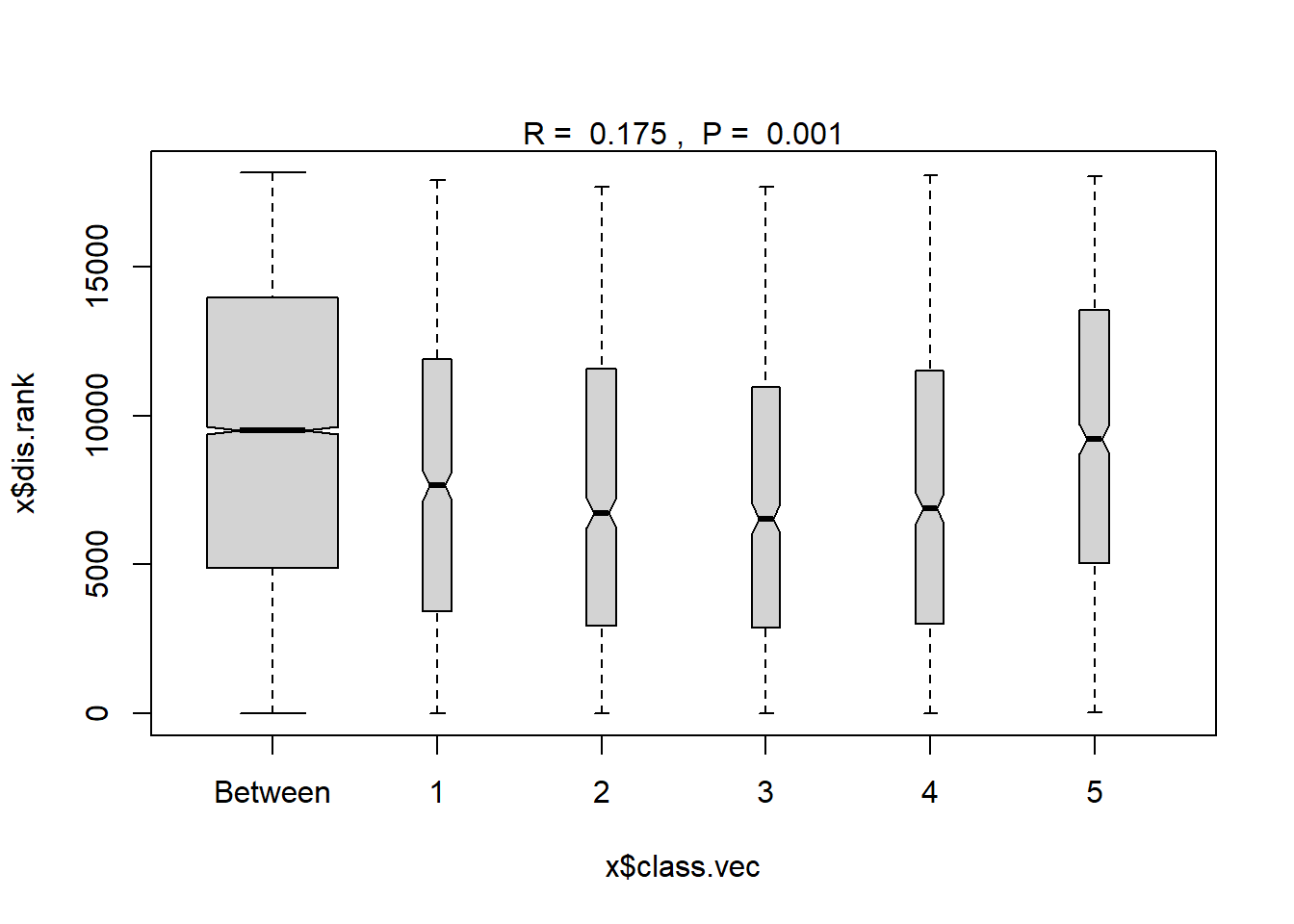
Region grouped
#region
ano_region_groups<- anosim(trawl_dist, trawl_data_arrange$REGION_NEW, permutations = 999)
ano_region_groups #regions are statistically different communities ##
## Call:
## anosim(x = trawl_dist, grouping = trawl_data_arrange$REGION_NEW, permutations = 999)
## Dissimilarity: bray
##
## ANOSIM statistic R: 0.02348
## Significance: 0.054
##
## Permutation: free
## Number of permutations: 999summary(ano_region_groups)##
## Call:
## anosim(x = trawl_dist, grouping = trawl_data_arrange$REGION_NEW, permutations = 999)
## Dissimilarity: bray
##
## ANOSIM statistic R: 0.02348
## Significance: 0.054
##
## Permutation: free
## Number of permutations: 999
##
## Upper quantiles of permutations (null model):
## 90% 95% 97.5% 99%
## 0.0183 0.0245 0.0300 0.0363
##
## Dissimilarity ranks between and within classes:
## 0% 25% 50% 75% 100% N
## Between 1 4642.25 9170.0 13694.25 18142 11626
## East of Penobscot Bay 17 5473.75 10428.0 14887.50 18145 2850
## Penobscot Bay 10 2901.00 6546.5 10943.75 17683 666
## West of Penobscot Bay 4 3809.50 8106.0 12484.50 18109 3003plot(ano_region_groups) #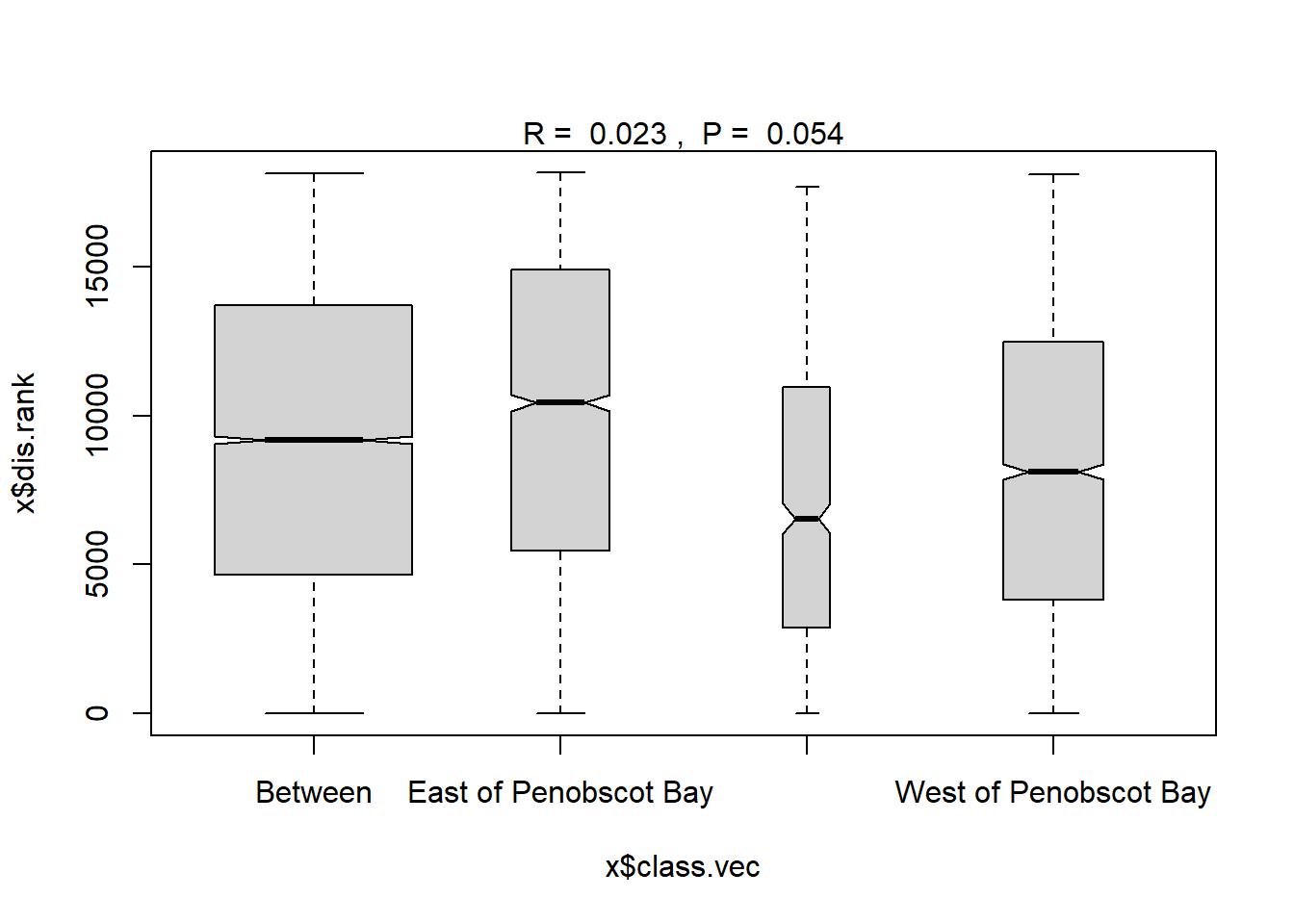
Year
#Time
ano_year<- anosim(trawl_dist, trawl_data_arrange$Year, permutations = 999)
ano_year #years are statistically different communities##
## Call:
## anosim(x = trawl_dist, grouping = trawl_data_arrange$Year, permutations = 999)
## Dissimilarity: bray
##
## ANOSIM statistic R: 0.2162
## Significance: 0.001
##
## Permutation: free
## Number of permutations: 999summary(ano_year)##
## Call:
## anosim(x = trawl_dist, grouping = trawl_data_arrange$Year, permutations = 999)
## Dissimilarity: bray
##
## ANOSIM statistic R: 0.2162
## Significance: 0.001
##
## Permutation: free
## Number of permutations: 999
##
## Upper quantiles of permutations (null model):
## 90% 95% 97.5% 99%
## 0.0233 0.0313 0.0379 0.0502
##
## Dissimilarity ranks between and within classes:
## 0% 25% 50% 75% 100% N
## Between 1 4650.50 9189.0 13698.50 18145 17315
## 2000 1504 3869.50 9400.0 11190.25 11685 10
## 2001 151 2783.00 10373.0 15110.00 17572 45
## 2002 262 5777.00 13093.0 17553.00 18142 45
## 2003 356 5570.00 9714.0 12017.00 16773 45
## 2004 321 5459.00 9695.0 12834.00 17641 45
## 2005 120 1704.00 3396.0 7352.00 17410 45
## 2006 97 2535.00 5928.0 11810.00 15577 45
## 2007 150 5050.00 7645.0 13112.00 17606 45
## 2008 11 2000.00 4588.0 10757.00 17061 45
## 2009 25 1148.00 3506.0 8587.00 16069 45
## 2010 318 3242.00 7116.0 11990.00 16823 45
## 2011 2 3754.00 6950.0 13440.00 16924 45
## 2012 512 2488.00 5540.0 10777.00 15354 45
## 2013 50 1978.00 4685.0 8730.00 12999 45
## 2014 125 4368.00 8423.0 10261.00 14762 45
## 2015 399 2225.00 5683.0 9243.00 14931 45
## 2016 384 3448.75 6346.5 9659.25 14780 28
## 2017 128 877.75 2415.5 4638.25 7011 36
## 2018 87 2901.00 8080.0 11820.00 15719 45
## 2019 249 2087.00 5031.5 9283.50 14875 36plot(ano_year)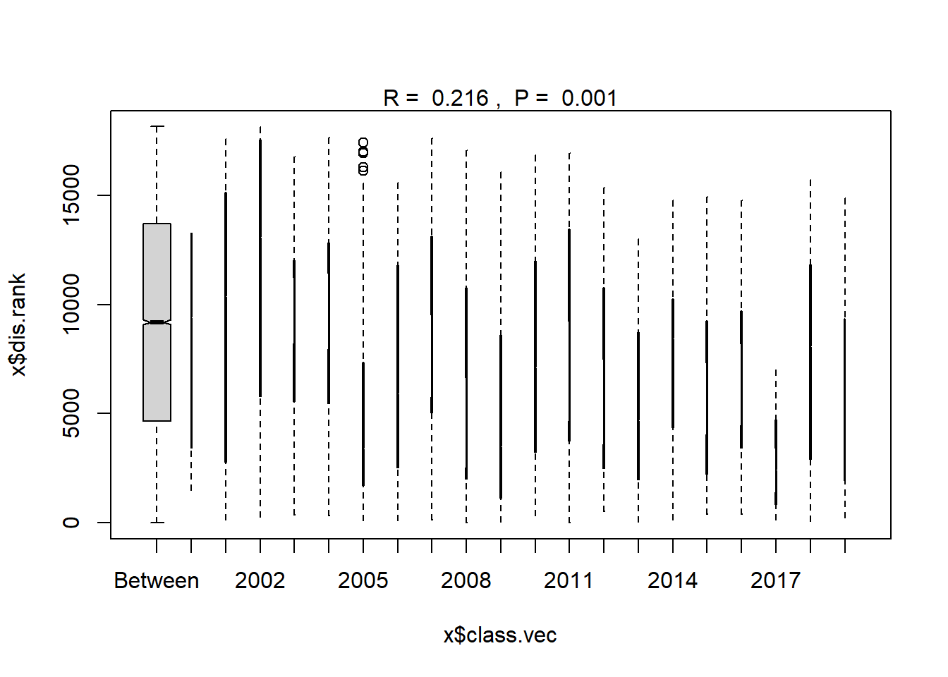
Year blocks
#Year blocks
ano_year_blocks<- anosim(trawl_dist, trawl_data_arrange$YEAR_GROUPS, permutations = 999)
ano_year_blocks #years are statistically different communities##
## Call:
## anosim(x = trawl_dist, grouping = trawl_data_arrange$YEAR_GROUPS, permutations = 999)
## Dissimilarity: bray
##
## ANOSIM statistic R: 0.1928
## Significance: 0.001
##
## Permutation: free
## Number of permutations: 999summary(ano_year_blocks)##
## Call:
## anosim(x = trawl_dist, grouping = trawl_data_arrange$YEAR_GROUPS, permutations = 999)
## Dissimilarity: bray
##
## ANOSIM statistic R: 0.1928
## Significance: 0.001
##
## Permutation: free
## Number of permutations: 999
##
## Upper quantiles of permutations (null model):
## 90% 95% 97.5% 99%
## 0.0123 0.0162 0.0197 0.0246
##
## Dissimilarity ranks between and within classes:
## 0% 25% 50% 75% 100% N
## Between 1 5064.0 9699.5 14069.75 18144 13670
## 2000-2004 15 5163.0 9414.5 13657.50 18145 990
## 2005-2009 4 2246.0 5569.0 10510.00 17977 1225
## 2010-2014 2 4018.0 8336.0 12782.00 17989 1225
## 2015-2019 20 2723.5 6034.0 10175.50 17646 1035plot(ano_year_blocks)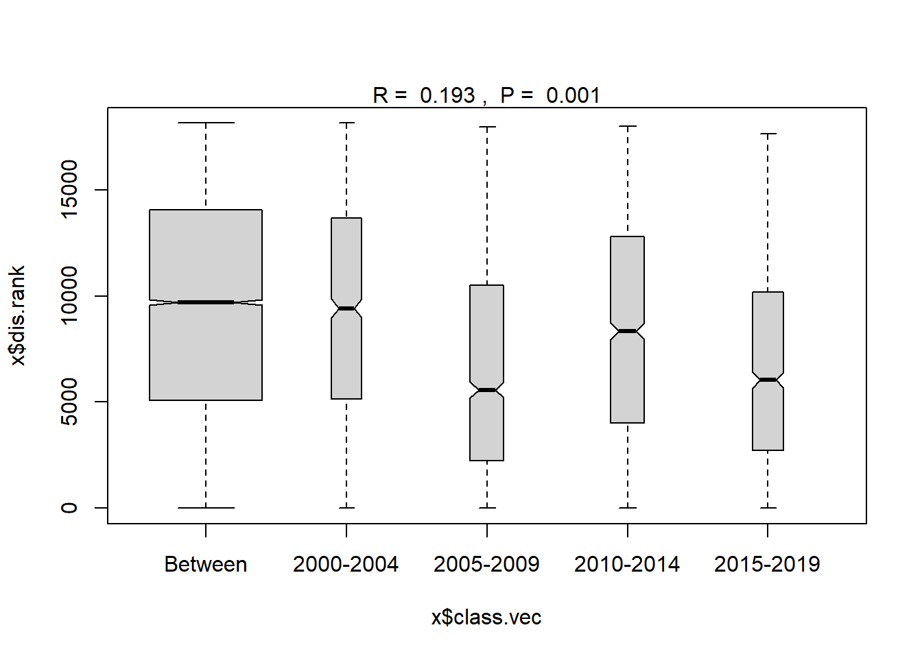
Analysis of variance (Adonis)
- Permanova
- tests whether there is a difference between means of groups
- works by calculating the sum of squares from the centroid of the group
Region and Year
adonis<-adonis2(trawl_dist~Region*Year, data=ME_group_data, by="terms", permutations = 9999)
adonis## Permutation test for adonis under reduced model
## Terms added sequentially (first to last)
## Permutation: free
## Number of permutations: 9999
##
## adonis2(formula = trawl_dist ~ Region * Year, data = ME_group_data, permutations = 9999, by = "terms")
## Df SumOfSqs R2 F Pr(>F)
## Region 1 0.3386 0.01404 2.7910 0.0374 *
## Year 1 0.8576 0.03557 7.0692 0.0007 ***
## Region:Year 1 0.2278 0.00945 1.8778 0.1232
## Residual 187 22.6859 0.94094
## Total 190 24.1099 1.00000
## ---
## Signif. codes: 0 '***' 0.001 '**' 0.01 '*' 0.05 '.' 0.1 ' ' 1summary(adonis)## Df SumOfSqs R2 F
## Min. : 1 Min. : 0.2278 Min. :0.009449 Min. :1.878
## 1st Qu.: 1 1st Qu.: 0.3386 1st Qu.:0.014044 1st Qu.:2.334
## Median : 1 Median : 0.8576 Median :0.035570 Median :2.791
## Mean : 76 Mean : 9.6440 Mean :0.400000 Mean :3.913
## 3rd Qu.:187 3rd Qu.:22.6859 3rd Qu.:0.940937 3rd Qu.:4.930
## Max. :190 Max. :24.1099 Max. :1.000000 Max. :7.069
## NA's :2
## Pr(>F)
## Min. :0.00070
## 1st Qu.:0.01905
## Median :0.03740
## Mean :0.05377
## 3rd Qu.:0.08030
## Max. :0.12320
## NA's :2Region
adonis<-adonis2(trawl_dist~Region, data=ME_group_data, by="terms", permutations = 9999)
adonis## Permutation test for adonis under reduced model
## Terms added sequentially (first to last)
## Permutation: free
## Number of permutations: 9999
##
## adonis2(formula = trawl_dist ~ Region, data = ME_group_data, permutations = 9999, by = "terms")
## Df SumOfSqs R2 F Pr(>F)
## Region 1 0.3386 0.01404 2.6921 0.0412 *
## Residual 189 23.7713 0.98596
## Total 190 24.1099 1.00000
## ---
## Signif. codes: 0 '***' 0.001 '**' 0.01 '*' 0.05 '.' 0.1 ' ' 1summary(adonis)## Df SumOfSqs R2 F
## Min. : 1.0 Min. : 0.3386 Min. :0.01404 Min. :2.692
## 1st Qu.: 95.0 1st Qu.:12.0550 1st Qu.:0.50000 1st Qu.:2.692
## Median :189.0 Median :23.7713 Median :0.98596 Median :2.692
## Mean :126.7 Mean :16.0733 Mean :0.66667 Mean :2.692
## 3rd Qu.:189.5 3rd Qu.:23.9406 3rd Qu.:0.99298 3rd Qu.:2.692
## Max. :190.0 Max. :24.1099 Max. :1.00000 Max. :2.692
## NA's :2
## Pr(>F)
## Min. :0.0412
## 1st Qu.:0.0412
## Median :0.0412
## Mean :0.0412
## 3rd Qu.:0.0412
## Max. :0.0412
## NA's :2Year
adonis<-adonis2(trawl_dist~Year, data=ME_group_data, by="terms", permutations = 9999)
adonis## Permutation test for adonis under reduced model
## Terms added sequentially (first to last)
## Permutation: free
## Number of permutations: 9999
##
## adonis2(formula = trawl_dist ~ Year, data = ME_group_data, permutations = 9999, by = "terms")
## Df SumOfSqs R2 F Pr(>F)
## Year 1 0.8586 0.03561 6.979 3e-04 ***
## Residual 189 23.2513 0.96439
## Total 190 24.1099 1.00000
## ---
## Signif. codes: 0 '***' 0.001 '**' 0.01 '*' 0.05 '.' 0.1 ' ' 1summary(adonis)## Df SumOfSqs R2 F
## Min. : 1.0 Min. : 0.8586 Min. :0.03561 Min. :6.979
## 1st Qu.: 95.0 1st Qu.:12.0550 1st Qu.:0.50000 1st Qu.:6.979
## Median :189.0 Median :23.2513 Median :0.96439 Median :6.979
## Mean :126.7 Mean :16.0733 Mean :0.66667 Mean :6.979
## 3rd Qu.:189.5 3rd Qu.:23.6806 3rd Qu.:0.98219 3rd Qu.:6.979
## Max. :190.0 Max. :24.1099 Max. :1.00000 Max. :6.979
## NA's :2
## Pr(>F)
## Min. :3e-04
## 1st Qu.:3e-04
## Median :3e-04
## Mean :3e-04
## 3rd Qu.:3e-04
## Max. :3e-04
## NA's :2Year block
#with year blocks
adonis<-adonis2(trawl_dist~YEAR_GROUPS, data=ME_group_data, by="terms", permutations = 9999)
adonis## Permutation test for adonis under reduced model
## Terms added sequentially (first to last)
## Permutation: free
## Number of permutations: 9999
##
## adonis2(formula = trawl_dist ~ YEAR_GROUPS, data = ME_group_data, permutations = 9999, by = "terms")
## Df SumOfSqs R2 F Pr(>F)
## YEAR_GROUPS 3 4.2949 0.17814 13.511 1e-04 ***
## Residual 187 19.8150 0.82186
## Total 190 24.1099 1.00000
## ---
## Signif. codes: 0 '***' 0.001 '**' 0.01 '*' 0.05 '.' 0.1 ' ' 1summary(adonis)## Df SumOfSqs R2 F
## Min. : 3.0 Min. : 4.295 Min. :0.1781 Min. :13.51
## 1st Qu.: 95.0 1st Qu.:12.055 1st Qu.:0.5000 1st Qu.:13.51
## Median :187.0 Median :19.815 Median :0.8219 Median :13.51
## Mean :126.7 Mean :16.073 Mean :0.6667 Mean :13.51
## 3rd Qu.:188.5 3rd Qu.:21.962 3rd Qu.:0.9109 3rd Qu.:13.51
## Max. :190.0 Max. :24.110 Max. :1.0000 Max. :13.51
## NA's :2
## Pr(>F)
## Min. :1e-04
## 1st Qu.:1e-04
## Median :1e-04
## Mean :1e-04
## 3rd Qu.:1e-04
## Max. :1e-04
## NA's :2Region and year block
#with year blocks
adonis<-adonis2(trawl_dist~Region*YEAR_GROUPS, data=ME_group_data, by="terms", permutations = 9999)
adonis## Permutation test for adonis under reduced model
## Terms added sequentially (first to last)
## Permutation: free
## Number of permutations: 9999
##
## adonis2(formula = trawl_dist ~ Region * YEAR_GROUPS, data = ME_group_data, permutations = 9999, by = "terms")
## Df SumOfSqs R2 F Pr(>F)
## Region 1 0.3386 0.01404 3.2364 0.0198 *
## YEAR_GROUPS 3 4.2999 0.17834 13.6997 0.0001 ***
## Region:YEAR_GROUPS 3 0.3257 0.01351 1.0377 0.4025
## Residual 183 19.1458 0.79410
## Total 190 24.1099 1.00000
## ---
## Signif. codes: 0 '***' 0.001 '**' 0.01 '*' 0.05 '.' 0.1 ' ' 1summary(adonis)## Df SumOfSqs R2 F
## Min. : 1 Min. : 0.3257 Min. :0.01351 Min. : 1.038
## 1st Qu.: 3 1st Qu.: 0.3386 1st Qu.:0.01404 1st Qu.: 2.137
## Median : 3 Median : 4.2999 Median :0.17834 Median : 3.236
## Mean : 76 Mean : 9.6440 Mean :0.40000 Mean : 5.991
## 3rd Qu.:183 3rd Qu.:19.1458 3rd Qu.:0.79410 3rd Qu.: 8.468
## Max. :190 Max. :24.1099 Max. :1.00000 Max. :13.700
## NA's :2
## Pr(>F)
## Min. :0.00010
## 1st Qu.:0.00995
## Median :0.01980
## Mean :0.14080
## 3rd Qu.:0.21115
## Max. :0.40250
## NA's :2Region groups
#with year blocks
adonis<-adonis2(trawl_dist~REGION_NEW, data=ME_group_data, by="terms", permutations = 9999)
adonis## Permutation test for adonis under reduced model
## Terms added sequentially (first to last)
## Permutation: free
## Number of permutations: 9999
##
## adonis2(formula = trawl_dist ~ REGION_NEW, data = ME_group_data, permutations = 9999, by = "terms")
## Df SumOfSqs R2 F Pr(>F)
## REGION_NEW 2 1.2003 0.04979 4.9251 4e-04 ***
## Residual 188 22.9096 0.95021
## Total 190 24.1099 1.00000
## ---
## Signif. codes: 0 '***' 0.001 '**' 0.01 '*' 0.05 '.' 0.1 ' ' 1summary(adonis)## Df SumOfSqs R2 F
## Min. : 2.0 Min. : 1.20 Min. :0.04979 Min. :4.925
## 1st Qu.: 95.0 1st Qu.:12.05 1st Qu.:0.50000 1st Qu.:4.925
## Median :188.0 Median :22.91 Median :0.95021 Median :4.925
## Mean :126.7 Mean :16.07 Mean :0.66667 Mean :4.925
## 3rd Qu.:189.0 3rd Qu.:23.51 3rd Qu.:0.97511 3rd Qu.:4.925
## Max. :190.0 Max. :24.11 Max. :1.00000 Max. :4.925
## NA's :2
## Pr(>F)
## Min. :4e-04
## 1st Qu.:4e-04
## Median :4e-04
## Mean :4e-04
## 3rd Qu.:4e-04
## Max. :4e-04
## NA's :2Region groups and year block
#with year blocks
adonis<-adonis2(trawl_dist~REGION_NEW*YEAR_GROUPS, data=ME_group_data, by="terms", permutations = 9999)
adonis## Permutation test for adonis under reduced model
## Terms added sequentially (first to last)
## Permutation: free
## Number of permutations: 9999
##
## adonis2(formula = trawl_dist ~ REGION_NEW * YEAR_GROUPS, data = ME_group_data, permutations = 9999, by = "terms")
## Df SumOfSqs R2 F Pr(>F)
## REGION_NEW 2 1.2003 0.04979 5.9172 0.0001 ***
## YEAR_GROUPS 3 4.2456 0.17610 13.9531 0.0001 ***
## REGION_NEW:YEAR_GROUPS 6 0.5086 0.02110 0.8358 0.6519
## Residual 179 18.1553 0.75302
## Total 190 24.1099 1.00000
## ---
## Signif. codes: 0 '***' 0.001 '**' 0.01 '*' 0.05 '.' 0.1 ' ' 1summary(adonis)## Df SumOfSqs R2 F
## Min. : 2 Min. : 0.5086 Min. :0.02110 Min. : 0.8358
## 1st Qu.: 3 1st Qu.: 1.2003 1st Qu.:0.04979 1st Qu.: 3.3765
## Median : 6 Median : 4.2456 Median :0.17610 Median : 5.9172
## Mean : 76 Mean : 9.6440 Mean :0.40000 Mean : 6.9020
## 3rd Qu.:179 3rd Qu.:18.1553 3rd Qu.:0.75302 3rd Qu.: 9.9352
## Max. :190 Max. :24.1099 Max. :1.00000 Max. :13.9531
## NA's :2
## Pr(>F)
## Min. :0.0001
## 1st Qu.:0.0001
## Median :0.0001
## Mean :0.2174
## 3rd Qu.:0.3260
## Max. :0.6519
## NA's :2Pairwise
- Vegan does not have a function for this, but I found a wrapper that seems frequently used on github
- select groups to test, one pair at a time
- Adjust p-values for multiple tests
Region
#pair-wise test to see what is different
pair<-pairwise.adonis2(trawl_dist~Region, data=ME_group_data, by="terms", permutations = 9999)
summary(pair)## Length Class Mode
## parent_call 1 -none- character
## 1_vs_2 6 anova list
## 1_vs_3 6 anova list
## 1_vs_4 6 anova list
## 1_vs_5 6 anova list
## 2_vs_3 6 anova list
## 2_vs_4 6 anova list
## 2_vs_5 6 anova list
## 3_vs_4 6 anova list
## 3_vs_5 6 anova list
## 4_vs_5 6 anova listpair ## $parent_call
## [1] "trawl_dist ~ Region , strata = Null"
##
## $`1_vs_2`
## Permutation: free
## Number of permutations: 9999
##
## Terms added sequentially (first to last)
##
## Df SumsOfSqs MeanSqs F.Model R2 Pr(>F)
## Region 1 0.9777 0.97771 9.7584 0.11379 1e-04 ***
## Residuals 76 7.6146 0.10019 0.88621
## Total 77 8.5923 1.00000
## ---
## Signif. codes: 0 '***' 0.001 '**' 0.01 '*' 0.05 '.' 0.1 ' ' 1
##
## $`1_vs_3`
## Permutation: free
## Number of permutations: 9999
##
## Terms added sequentially (first to last)
##
## Df SumsOfSqs MeanSqs F.Model R2 Pr(>F)
## Region 1 1.5395 1.53951 15.639 0.17446 1e-04 ***
## Residuals 74 7.2847 0.09844 0.82554
## Total 75 8.8242 1.00000
## ---
## Signif. codes: 0 '***' 0.001 '**' 0.01 '*' 0.05 '.' 0.1 ' ' 1
##
## $`1_vs_4`
## Permutation: free
## Number of permutations: 9999
##
## Terms added sequentially (first to last)
##
## Df SumsOfSqs MeanSqs F.Model R2 Pr(>F)
## Region 1 1.5860 1.58600 15.243 0.1708 1e-04 ***
## Residuals 74 7.6997 0.10405 0.8292
## Total 75 9.2857 1.0000
## ---
## Signif. codes: 0 '***' 0.001 '**' 0.01 '*' 0.05 '.' 0.1 ' ' 1
##
## $`1_vs_5`
## Permutation: free
## Number of permutations: 9999
##
## Terms added sequentially (first to last)
##
## Df SumsOfSqs MeanSqs F.Model R2 Pr(>F)
## Region 1 0.3896 0.38965 3.3956 0.04277 0.0136 *
## Residuals 76 8.7210 0.11475 0.95723
## Total 77 9.1106 1.00000
## ---
## Signif. codes: 0 '***' 0.001 '**' 0.01 '*' 0.05 '.' 0.1 ' ' 1
##
## $`2_vs_3`
## Permutation: free
## Number of permutations: 9999
##
## Terms added sequentially (first to last)
##
## Df SumsOfSqs MeanSqs F.Model R2 Pr(>F)
## Region 1 0.1162 0.116214 1.2349 0.01641 0.2883
## Residuals 74 6.9640 0.094108 0.98359
## Total 75 7.0802 1.00000
##
## $`2_vs_4`
## Permutation: free
## Number of permutations: 9999
##
## Terms added sequentially (first to last)
##
## Df SumsOfSqs MeanSqs F.Model R2 Pr(>F)
## Region 1 0.1733 0.173297 1.7379 0.02295 0.1488
## Residuals 74 7.3790 0.099716 0.97705
## Total 75 7.5523 1.00000
##
## $`2_vs_5`
## Permutation: free
## Number of permutations: 9999
##
## Terms added sequentially (first to last)
##
## Df SumsOfSqs MeanSqs F.Model R2 Pr(>F)
## Region 1 1.8959 1.89593 17.153 0.18414 1e-04 ***
## Residuals 76 8.4002 0.11053 0.81586
## Total 77 10.2962 1.00000
## ---
## Signif. codes: 0 '***' 0.001 '**' 0.01 '*' 0.05 '.' 0.1 ' ' 1
##
## $`3_vs_4`
## Permutation: free
## Number of permutations: 9999
##
## Terms added sequentially (first to last)
##
## Df SumsOfSqs MeanSqs F.Model R2 Pr(>F)
## Region 1 0.0318 0.031804 0.32485 0.00449 0.8207
## Residuals 72 7.0491 0.097904 0.99551
## Total 73 7.0809 1.00000
##
## $`3_vs_5`
## Permutation: free
## Number of permutations: 9999
##
## Terms added sequentially (first to last)
##
## Df SumsOfSqs MeanSqs F.Model R2 Pr(>F)
## Region 1 2.4840 2.48400 22.777 0.23535 1e-04 ***
## Residuals 74 8.0704 0.10906 0.76465
## Total 75 10.5543 1.00000
## ---
## Signif. codes: 0 '***' 0.001 '**' 0.01 '*' 0.05 '.' 0.1 ' ' 1
##
## $`4_vs_5`
## Permutation: free
## Number of permutations: 9999
##
## Terms added sequentially (first to last)
##
## Df SumsOfSqs MeanSqs F.Model R2 Pr(>F)
## Region 1 2.5149 2.51486 21.932 0.22862 1e-04 ***
## Residuals 74 8.4854 0.11467 0.77138
## Total 75 11.0002 1.00000
## ---
## Signif. codes: 0 '***' 0.001 '**' 0.01 '*' 0.05 '.' 0.1 ' ' 1
##
## attr(,"class")
## [1] "pwadstrata" "list"Region groups
#pair-wise test to see what is different
pair<-pairwise.adonis2(trawl_dist~REGION_NEW, data=ME_group_data, by="terms", permutations = 9999)
summary(pair)## Length Class Mode
## parent_call 1 -none- character
## West of Penobscot Bay_vs_Penobscot Bay 6 anova list
## West of Penobscot Bay_vs_East of Penobscot Bay 6 anova list
## Penobscot Bay_vs_East of Penobscot Bay 6 anova listpair ## $parent_call
## [1] "trawl_dist ~ REGION_NEW , strata = Null"
##
## $`West of Penobscot Bay_vs_Penobscot Bay`
## Permutation: free
## Number of permutations: 9999
##
## Terms added sequentially (first to last)
##
## Df SumsOfSqs MeanSqs F.Model R2 Pr(>F)
## REGION_NEW 1 0.7796 0.77965 7.3976 0.06144 1e-04 ***
## Residuals 113 11.9094 0.10539 0.93856
## Total 114 12.6890 1.00000
## ---
## Signif. codes: 0 '***' 0.001 '**' 0.01 '*' 0.05 '.' 0.1 ' ' 1
##
## $`West of Penobscot Bay_vs_East of Penobscot Bay`
## Permutation: free
## Number of permutations: 9999
##
## Terms added sequentially (first to last)
##
## Df SumsOfSqs MeanSqs F.Model R2 Pr(>F)
## REGION_NEW 1 0.2696 0.26959 2.0915 0.01357 0.0878 .
## Residuals 152 19.5925 0.12890 0.98643
## Total 153 19.8621 1.00000
## ---
## Signif. codes: 0 '***' 0.001 '**' 0.01 '*' 0.05 '.' 0.1 ' ' 1
##
## $`Penobscot Bay_vs_East of Penobscot Bay`
## Permutation: free
## Number of permutations: 9999
##
## Terms added sequentially (first to last)
##
## Df SumsOfSqs MeanSqs F.Model R2 Pr(>F)
## REGION_NEW 1 0.868 0.86803 6.7297 0.05716 6e-04 ***
## Residuals 111 14.317 0.12898 0.94284
## Total 112 15.185 1.00000
## ---
## Signif. codes: 0 '***' 0.001 '**' 0.01 '*' 0.05 '.' 0.1 ' ' 1
##
## attr(,"class")
## [1] "pwadstrata" "list"Year blocks
#pair-wise test to see what is different for year blocks
pair<-pairwise.adonis2(trawl_dist~YEAR_GROUPS, data=ME_group_data, by="terms", permutations = 9999)
summary(pair)## Length Class Mode
## parent_call 1 -none- character
## 2000-2004_vs_2005-2009 6 anova list
## 2000-2004_vs_2010-2014 6 anova list
## 2000-2004_vs_2015-2019 6 anova list
## 2005-2009_vs_2010-2014 6 anova list
## 2005-2009_vs_2015-2019 6 anova list
## 2010-2014_vs_2015-2019 6 anova listpair## $parent_call
## [1] "trawl_dist ~ YEAR_GROUPS , strata = Null"
##
## $`2000-2004_vs_2005-2009`
## Permutation: free
## Number of permutations: 9999
##
## Terms added sequentially (first to last)
##
## Df SumsOfSqs MeanSqs F.Model R2 Pr(>F)
## YEAR_GROUPS 1 2.3191 2.31911 20.739 0.18234 1e-04 ***
## Residuals 93 10.3995 0.11182 0.81766
## Total 94 12.7186 1.00000
## ---
## Signif. codes: 0 '***' 0.001 '**' 0.01 '*' 0.05 '.' 0.1 ' ' 1
##
## $`2000-2004_vs_2010-2014`
## Permutation: free
## Number of permutations: 9999
##
## Terms added sequentially (first to last)
##
## Df SumsOfSqs MeanSqs F.Model R2 Pr(>F)
## YEAR_GROUPS 1 0.4762 0.47622 3.8334 0.03959 0.0072 **
## Residuals 93 11.5534 0.12423 0.96041
## Total 94 12.0297 1.00000
## ---
## Signif. codes: 0 '***' 0.001 '**' 0.01 '*' 0.05 '.' 0.1 ' ' 1
##
## $`2000-2004_vs_2015-2019`
## Permutation: free
## Number of permutations: 9999
##
## Terms added sequentially (first to last)
##
## Df SumsOfSqs MeanSqs F.Model R2 Pr(>F)
## YEAR_GROUPS 1 0.3524 0.35245 3.1907 0.03461 0.0228 *
## Residuals 89 9.8311 0.11046 0.96539
## Total 90 10.1836 1.00000
## ---
## Signif. codes: 0 '***' 0.001 '**' 0.01 '*' 0.05 '.' 0.1 ' ' 1
##
## $`2005-2009_vs_2010-2014`
## Permutation: free
## Number of permutations: 9999
##
## Terms added sequentially (first to last)
##
## Df SumsOfSqs MeanSqs F.Model R2 Pr(>F)
## YEAR_GROUPS 1 1.3748 1.37482 13.495 0.12104 1e-04 ***
## Residuals 98 9.9839 0.10188 0.87896
## Total 99 11.3587 1.00000
## ---
## Signif. codes: 0 '***' 0.001 '**' 0.01 '*' 0.05 '.' 0.1 ' ' 1
##
## $`2005-2009_vs_2015-2019`
## Permutation: free
## Number of permutations: 9999
##
## Terms added sequentially (first to last)
##
## Df SumsOfSqs MeanSqs F.Model R2 Pr(>F)
## YEAR_GROUPS 1 3.3133 3.3133 37.698 0.28625 1e-04 ***
## Residuals 94 8.2616 0.0879 0.71375
## Total 95 11.5748 1.00000
## ---
## Signif. codes: 0 '***' 0.001 '**' 0.01 '*' 0.05 '.' 0.1 ' ' 1
##
## $`2010-2014_vs_2015-2019`
## Permutation: free
## Number of permutations: 9999
##
## Terms added sequentially (first to last)
##
## Df SumsOfSqs MeanSqs F.Model R2 Pr(>F)
## YEAR_GROUPS 1 0.6994 0.69941 6.9826 0.06915 2e-04 ***
## Residuals 94 9.4155 0.10017 0.93085
## Total 95 10.1149 1.00000
## ---
## Signif. codes: 0 '***' 0.001 '**' 0.01 '*' 0.05 '.' 0.1 ' ' 1
##
## attr(,"class")
## [1] "pwadstrata" "list"Dispersion
- anosim very sensitive to heterogeneity (Anderson and Walsh 2013)
- Could get false significant results from differences in variance instead of mean
- adonis is less affected by heterogeneity for balanced designs
- PRIMER can deal with dispersion issues, but vegan does not yet
- tests null hypothesis that there is no difference in dispersion between groups
- p-value <0.05 means difference is significant
Region
#betadisper test homogeneity of dispersion among groups
#Region
bd<-betadisper(trawl_dist,ME_group_data$Region)
bd##
## Homogeneity of multivariate dispersions
##
## Call: betadisper(d = trawl_dist, group = ME_group_data$Region)
##
## No. of Positive Eigenvalues: 59
## No. of Negative Eigenvalues: 131
##
## Average distance to median:
## 1 2 3 4 5
## 0.3037 0.2908 0.2856 0.2899 0.3305
##
## Eigenvalues for PCoA axes:
## (Showing 8 of 190 eigenvalues)
## PCoA1 PCoA2 PCoA3 PCoA4 PCoA5 PCoA6 PCoA7 PCoA8
## 11.7246 5.3723 3.2034 2.4972 1.5778 1.0868 0.7343 0.6527anova(bd) ## Analysis of Variance Table
##
## Response: Distances
## Df Sum Sq Mean Sq F value Pr(>F)
## Groups 4 0.05142 0.012856 1.0394 0.3882
## Residuals 186 2.30058 0.012369#test based on permutations
permutest(bd)##
## Permutation test for homogeneity of multivariate dispersions
## Permutation: free
## Number of permutations: 999
##
## Response: Distances
## Df Sum Sq Mean Sq F N.Perm Pr(>F)
## Groups 4 0.05142 0.012856 1.0394 999 0.384
## Residuals 186 2.30058 0.012369plot(bd, hull=FALSE, ellipse = TRUE) 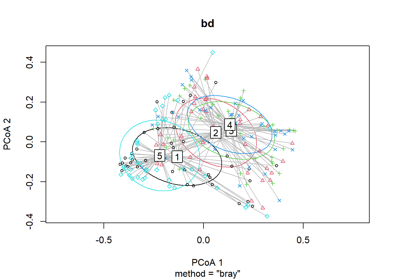
boxplot(bd)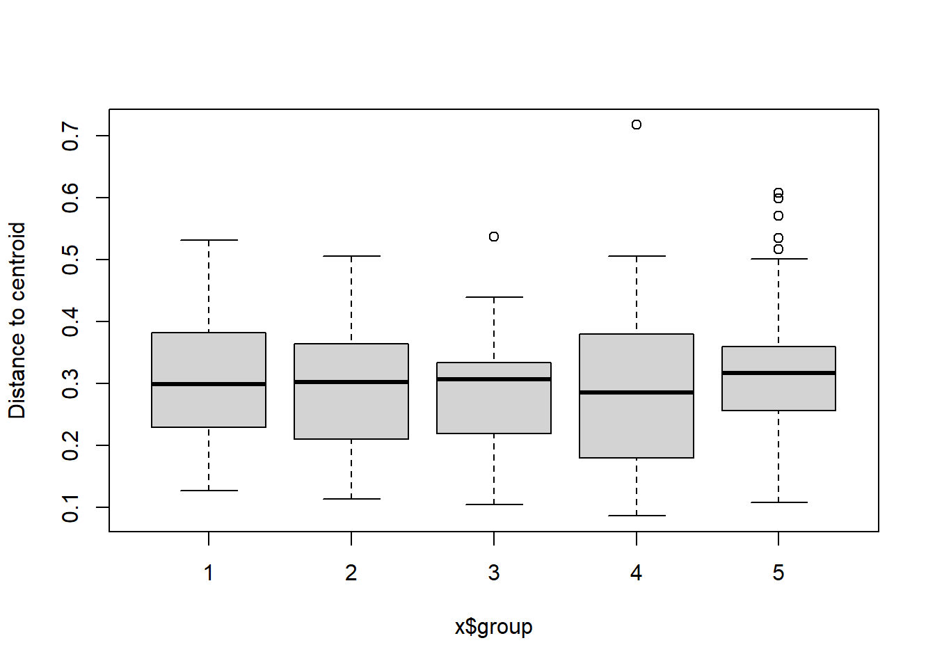
Region group
#Region
bd<-betadisper(trawl_dist,ME_group_data$REGION_NEW)
bd##
## Homogeneity of multivariate dispersions
##
## Call: betadisper(d = trawl_dist, group = ME_group_data$REGION_NEW)
##
## No. of Positive Eigenvalues: 59
## No. of Negative Eigenvalues: 131
##
## Average distance to median:
## East of Penobscot Bay Penobscot Bay West of Penobscot Bay
## 0.3659 0.2856 0.3164
##
## Eigenvalues for PCoA axes:
## (Showing 8 of 190 eigenvalues)
## PCoA1 PCoA2 PCoA3 PCoA4 PCoA5 PCoA6 PCoA7 PCoA8
## 11.7246 5.3723 3.2034 2.4972 1.5778 1.0868 0.7343 0.6527anova(bd) ## Analysis of Variance Table
##
## Response: Distances
## Df Sum Sq Mean Sq F value Pr(>F)
## Groups 2 0.18523 0.092613 8.6261 0.0002605 ***
## Residuals 188 2.01843 0.010736
## ---
## Signif. codes: 0 '***' 0.001 '**' 0.01 '*' 0.05 '.' 0.1 ' ' 1#test based on permutations
permutest(bd)##
## Permutation test for homogeneity of multivariate dispersions
## Permutation: free
## Number of permutations: 999
##
## Response: Distances
## Df Sum Sq Mean Sq F N.Perm Pr(>F)
## Groups 2 0.18523 0.092613 8.6261 999 0.001 ***
## Residuals 188 2.01843 0.010736
## ---
## Signif. codes: 0 '***' 0.001 '**' 0.01 '*' 0.05 '.' 0.1 ' ' 1plot(bd, hull=FALSE, ellipse = TRUE) 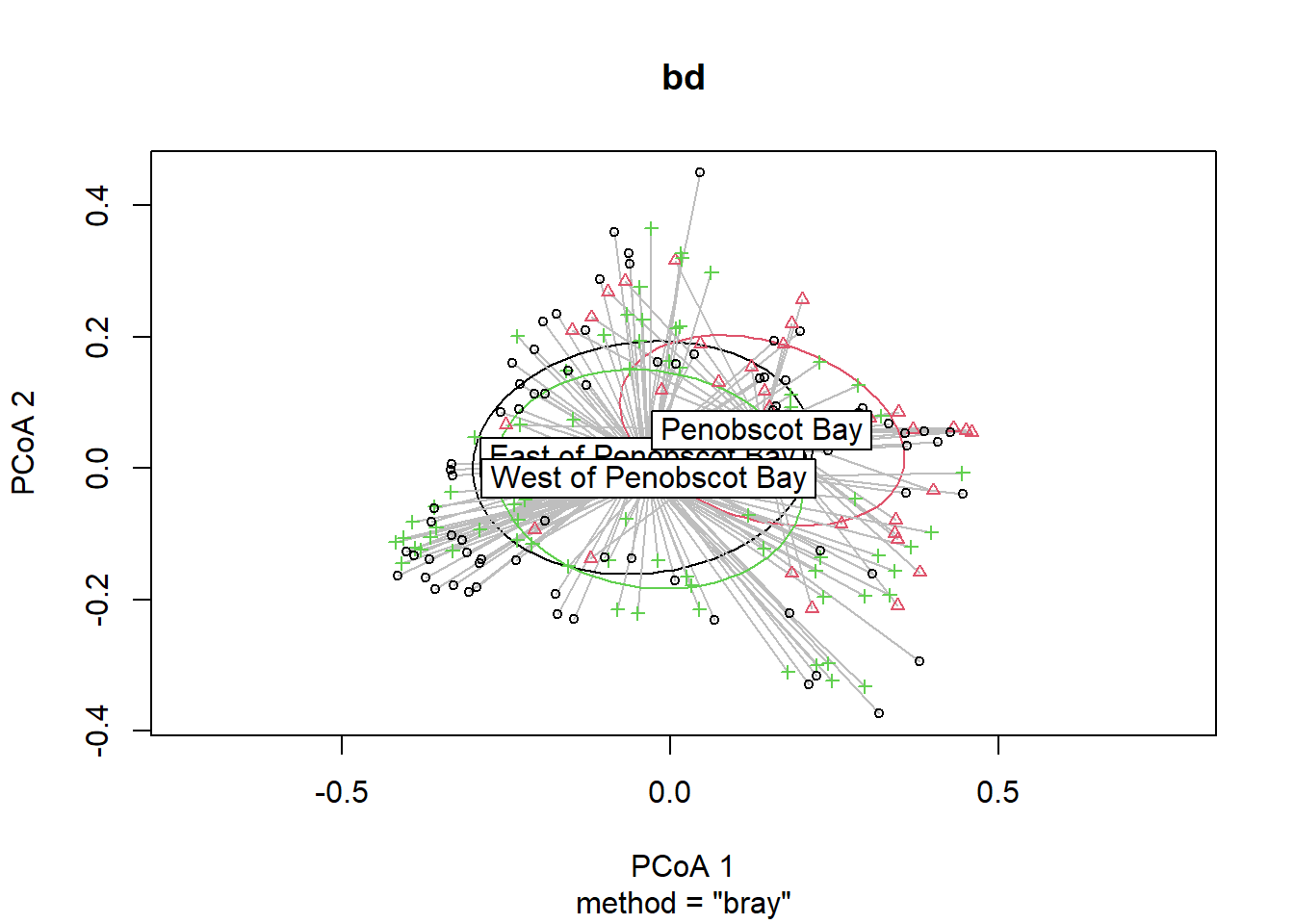
boxplot(bd)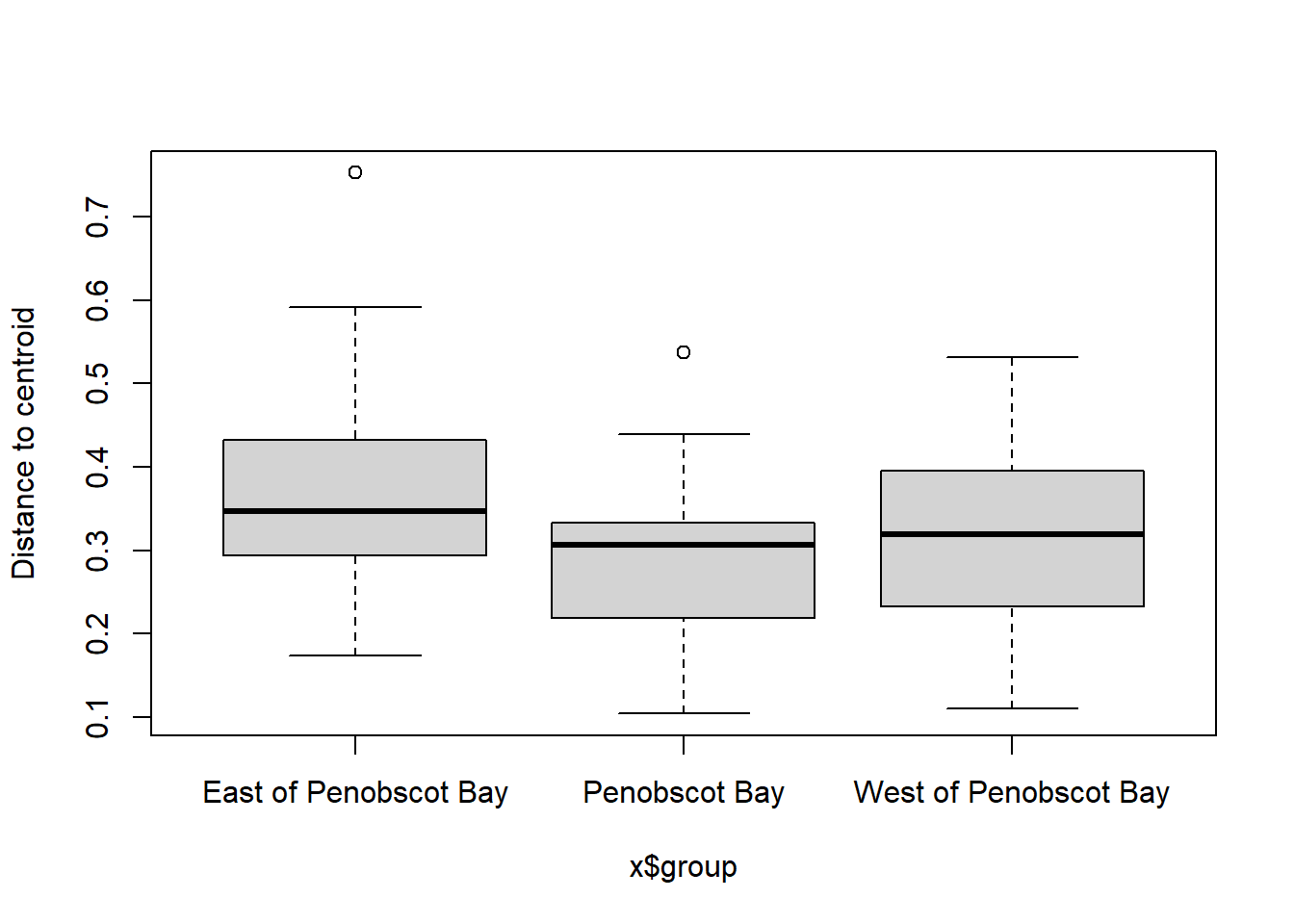
Year
#Year
bd<-betadisper(trawl_dist,ME_group_data$Year)
bd##
## Homogeneity of multivariate dispersions
##
## Call: betadisper(d = trawl_dist, group = ME_group_data$Year)
##
## No. of Positive Eigenvalues: 59
## No. of Negative Eigenvalues: 131
##
## Average distance to median:
## 2000 2001 2002 2003 2004 2005 2006 2007 2008 2009 2010
## 0.2522 0.3087 0.3622 0.3110 0.3101 0.2177 0.2642 0.3056 0.2376 0.2119 0.2807
## 2011 2012 2013 2014 2015 2016 2017 2018 2019
## 0.2908 0.2690 0.2353 0.2841 0.2451 0.2539 0.1616 0.2843 0.2403
##
## Eigenvalues for PCoA axes:
## (Showing 8 of 190 eigenvalues)
## PCoA1 PCoA2 PCoA3 PCoA4 PCoA5 PCoA6 PCoA7 PCoA8
## 11.7246 5.3723 3.2034 2.4972 1.5778 1.0868 0.7343 0.6527anova(bd) ## Analysis of Variance Table
##
## Response: Distances
## Df Sum Sq Mean Sq F value Pr(>F)
## Groups 19 0.36137 0.019020 1.1103 0.3445
## Residuals 171 2.92939 0.017131#test based on permutations
permutest(bd)##
## Permutation test for homogeneity of multivariate dispersions
## Permutation: free
## Number of permutations: 999
##
## Response: Distances
## Df Sum Sq Mean Sq F N.Perm Pr(>F)
## Groups 19 0.36137 0.019020 1.1103 999 0.384
## Residuals 171 2.92939 0.017131plot(bd, hull=FALSE, ellipse = TRUE)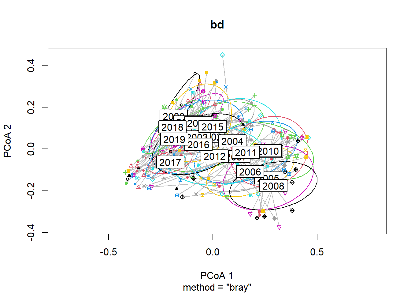
boxplot(bd)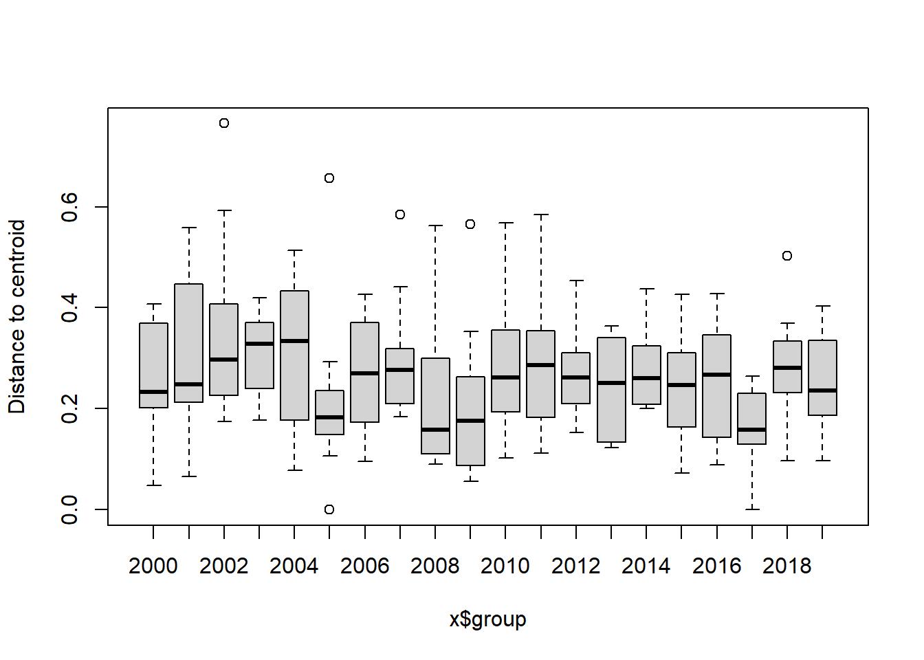
Year block
#Year blocks
bd<-betadisper(trawl_dist,ME_group_data$YEAR_GROUPS)
bd##
## Homogeneity of multivariate dispersions
##
## Call: betadisper(d = trawl_dist, group = ME_group_data$YEAR_GROUPS)
##
## No. of Positive Eigenvalues: 59
## No. of Negative Eigenvalues: 131
##
## Average distance to median:
## 2000-2004 2005-2009 2010-2014 2015-2019
## 0.3443 0.2706 0.3162 0.2728
##
## Eigenvalues for PCoA axes:
## (Showing 8 of 190 eigenvalues)
## PCoA1 PCoA2 PCoA3 PCoA4 PCoA5 PCoA6 PCoA7 PCoA8
## 11.7246 5.3723 3.2034 2.4972 1.5778 1.0868 0.7343 0.6527anova(bd) ## Analysis of Variance Table
##
## Response: Distances
## Df Sum Sq Mean Sq F value Pr(>F)
## Groups 3 0.17867 0.059557 4.2914 0.005898 **
## Residuals 187 2.59524 0.013878
## ---
## Signif. codes: 0 '***' 0.001 '**' 0.01 '*' 0.05 '.' 0.1 ' ' 1#test based on permutations
permutest(bd)##
## Permutation test for homogeneity of multivariate dispersions
## Permutation: free
## Number of permutations: 999
##
## Response: Distances
## Df Sum Sq Mean Sq F N.Perm Pr(>F)
## Groups 3 0.17867 0.059557 4.2914 999 0.006 **
## Residuals 187 2.59524 0.013878
## ---
## Signif. codes: 0 '***' 0.001 '**' 0.01 '*' 0.05 '.' 0.1 ' ' 1plot(bd, hull=FALSE, ellipse = TRUE)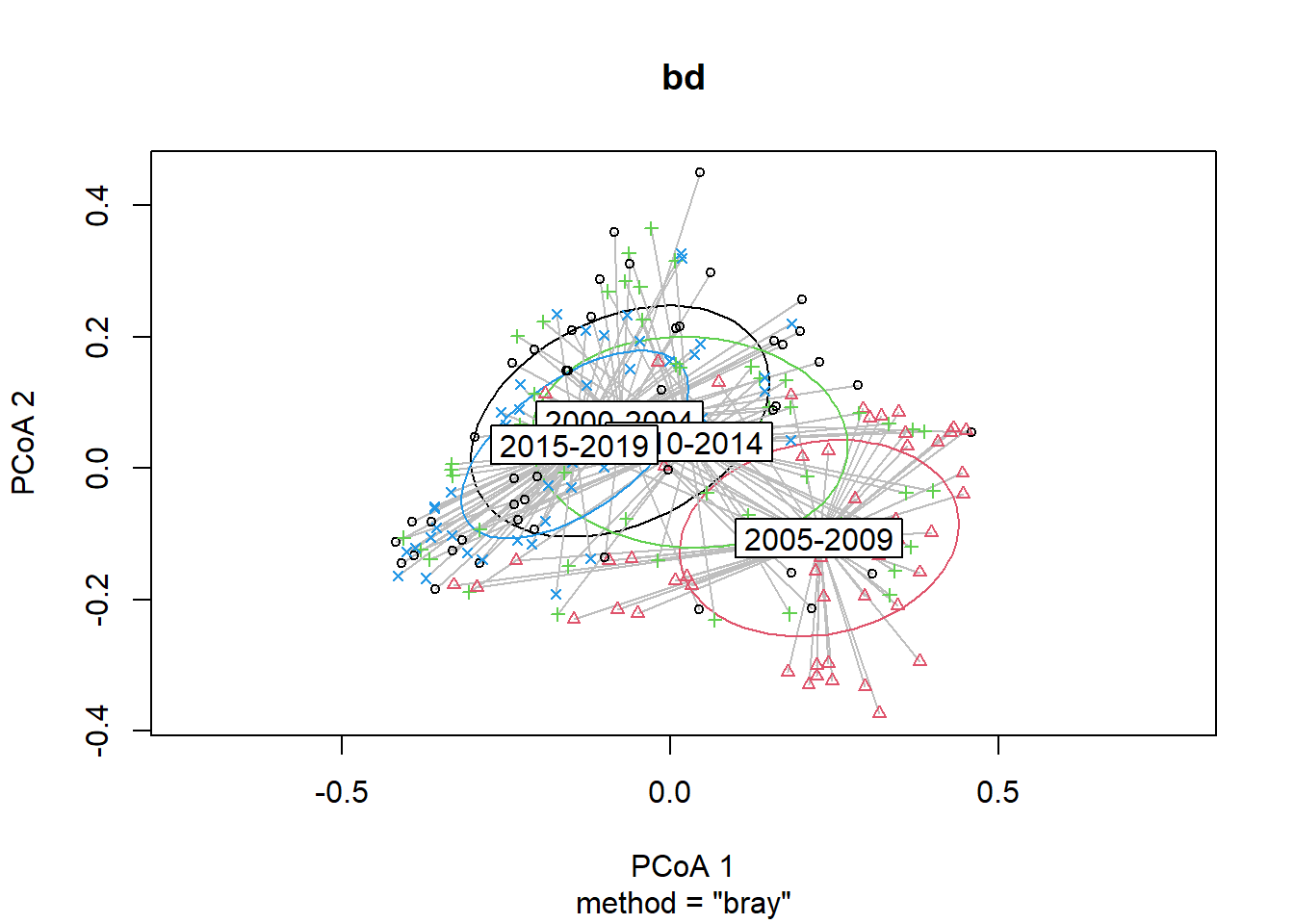
boxplot(bd)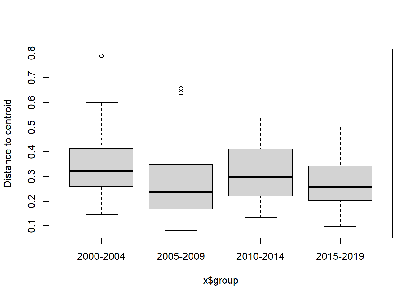
Indicator species analysis
- test if a species if found significantly more in one group compared to another
- all combinations of groups
Region
#see which species are found significantly more in each Region
inv_region<-multipatt(ME_NMDS_data, ME_group_data$Region, func = "r.g", control = how(nperm=999))
summary(inv_region)##
## Multilevel pattern analysis
## ---------------------------
##
## Association function: r.g
## Significance level (alpha): 0.05
##
## Total number of species: 5
## Selected number of species: 4
## Number of species associated to 1 group: 0
## Number of species associated to 2 groups: 1
## Number of species associated to 3 groups: 2
## Number of species associated to 4 groups: 1
##
## List of species associated to each combination:
##
## Group 4+5 #sps. 1
## stat p.value
## benthos 0.293 0.001 ***
##
## Group 2+3+4 #sps. 2
## stat p.value
## planktivore 0.539 0.001 ***
## undefined 0.322 0.001 ***
##
## Group 1+2+3+4 #sps. 1
## stat p.value
## piscivore 0.233 0.009 **
## ---
## Signif. codes: 0 '***' 0.001 '**' 0.01 '*' 0.05 '.' 0.1 ' ' 1Year block
#see which species are found significantly more in each Region
inv_year<-multipatt(ME_NMDS_data, ME_group_data$YEAR_GROUPS, func = "r.g", control = how(nperm=999))
summary(inv_year)##
## Multilevel pattern analysis
## ---------------------------
##
## Association function: r.g
## Significance level (alpha): 0.05
##
## Total number of species: 5
## Selected number of species: 4
## Number of species associated to 1 group: 1
## Number of species associated to 2 groups: 3
## Number of species associated to 3 groups: 0
##
## List of species associated to each combination:
##
## Group 2000-2004 #sps. 1
## stat p.value
## benthos 0.21 0.02 *
##
## Group 2005-2009+2010-2014 #sps. 1
## stat p.value
## undefined 0.313 0.001 ***
##
## Group 2010-2014+2015-2019 #sps. 2
## stat p.value
## benthivore 0.422 0.001 ***
## piscivore 0.282 0.001 ***
## ---
## Signif. codes: 0 '***' 0.001 '**' 0.01 '*' 0.05 '.' 0.1 ' ' 1