ME-NH trawl diveristy metrics

By season and total

library(here)
library(ggplot2)
library(dplyr)

setwd("C:/Users/jjesse/Desktop/GMRI/ME-NH-Trawl-Seagrant/Data")
new_data<-read.csv("MaineDMR_Trawl_Survey_Catch_Data_2021-05-14.csv")

#remove unnecessary species by getting scientific name from old data
setwd("C:/Users/jjesse/Box/Kerr Lab/Fisheries Science Lab/ME NH Trawl- Seagrant/Seagrant-AEW/ME NH data for GMRI")

trawl <- read.csv("EXPCATCH_forGMRI.csv", header = TRUE)%>%
  select(COMMON_NAME, SCIENTIFIC_NAME)%>%
  distinct()

trawl_2<- left_join(trawl,new_data)

# first drop samples that are not to the species level
trawl_2 <- trawl_2[!trawl_2$SCIENTIFIC_NAME == "Anemonia" ,]
trawl_2 <- trawl_2[!trawl_2$SCIENTIFIC_NAME == "Pandalus" ,]    #ID to spp also
trawl_2 <- trawl_2[!trawl_2$SCIENTIFIC_NAME == "Stelleroidea",]
trawl_2 <- trawl_2[!trawl_2$SCIENTIFIC_NAME == "Octopoda",]
trawl_2 <- trawl_2[!trawl_2$SCIENTIFIC_NAME == "Clypeasteroida",]
trawl_2 <- trawl_2[!trawl_2$SCIENTIFIC_NAME == "Yoldia",]
trawl_2 <- trawl_2[!trawl_2$SCIENTIFIC_NAME == "Calcarea",]
trawl_2 <- trawl_2[!trawl_2$SCIENTIFIC_NAME == "Majidae",]
trawl_2 <- trawl_2[!trawl_2$SCIENTIFIC_NAME == "Balanus",]
trawl_2 <- trawl_2[!trawl_2$SCIENTIFIC_NAME == "Stomatopoda",]    #low
trawl_2 <- trawl_2[!trawl_2$SCIENTIFIC_NAME == "Euphausiacea",]
trawl_2 <- trawl_2[!trawl_2$SCIENTIFIC_NAME == "Paguroidea",]
trawl_2 <- trawl_2[!trawl_2$SCIENTIFIC_NAME == "",]
trawl_2 <- trawl_2[!trawl_2$SCIENTIFIC_NAME == "Mysidacea",]
trawl_2 <- trawl_2[!trawl_2$SCIENTIFIC_NAME == "Diaphus",]        #low
trawl_2 <- trawl_2[!trawl_2$SCIENTIFIC_NAME == "Sepiolidae",]
trawl_2 <- trawl_2[!trawl_2$SCIENTIFIC_NAME == "Artediellus",]    #low
trawl_2 <- trawl_2[!trawl_2$SCIENTIFIC_NAME == "Macrouridae",]    #low
trawl_2 <- trawl_2[!trawl_2$SCIENTIFIC_NAME == "Paralepididae",]  #low
trawl_2 <- trawl_2[!trawl_2$SCIENTIFIC_NAME == "Clupeidae",]      #low
trawl_2 <- trawl_2[!trawl_2$SCIENTIFIC_NAME == "Myctophidae",]    #low

## there are 1121 occurrences where catch = NA; remove these?
trawl_2 <- trawl_2[!is.na(trawl_2$Expanded_Catch),]
## for some reason there 26 are observations of catch = 0; remove these 
trawl_2 <- trawl_2[!trawl_2$Expanded_Catch == 0,]

## there are 16 occurrences where weight = NA; remove these?
trawl_2 <- trawl_2[!is.na(trawl_2$Expanded_Weight_kg),]
## for some reason there 0 are observations of weight = 0; remove these 
trawl_2 <- trawl_2[!trawl_2$Expanded_Catch == 0,]

data<-trawl_2

Species richness

me_richness<-group_by(data, Year,Season, Tow_Number)%>%
  summarise(richness=length(unique(COMMON_NAME)))%>%
  group_by(Year, Season)%>%
  summarise(avg_richness=mean(richness))

ggplot()+ geom_line(data=me_richness, aes(Year, avg_richness))+facet_grid(rows = vars(Season))+theme_bw()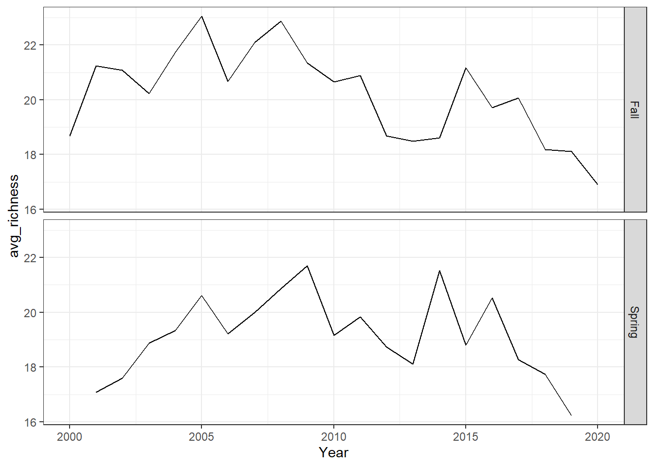

richness<-group_by(data, Year, Season, Tow_Number)%>%
  summarise(richness=length(unique(COMMON_NAME)))%>%
  group_by(Year)%>%
  summarise(avg_richness=mean(richness))

rich<-ggplot()+ geom_line(data=subset(richness,Year>2005 & Year<2020), aes(Year, avg_richness))+ theme_classic()+ ylab(expression(paste("Species\nRichness")))+theme(plot.margin = margin(10, 10, 10, 20))

rich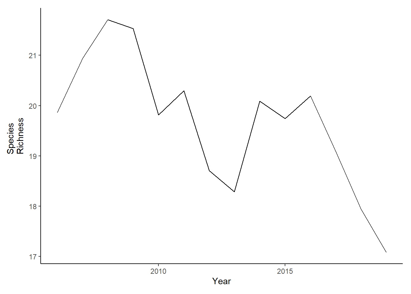

Shannon-Weiner diversity

me_shannon<-group_by(data, Year,Season, Tow_Number, COMMON_NAME)%>%
  mutate(species_total=sum(Expanded_Weight_kg, na.rm=TRUE))%>%
  group_by(Year, Season, Tow_Number)%>%
  mutate(total=sum(species_total), prop=(species_total/total))%>%
  summarise(shannon=-1*(sum(prop*log(prop),na.rm=TRUE)))%>%
  group_by(Year, Season)%>%
  summarise(avg_shannon=mean(shannon))

ggplot()+geom_line(data=me_shannon, aes(Year, avg_shannon))+ 
  facet_grid(rows=vars(Season))+theme_bw()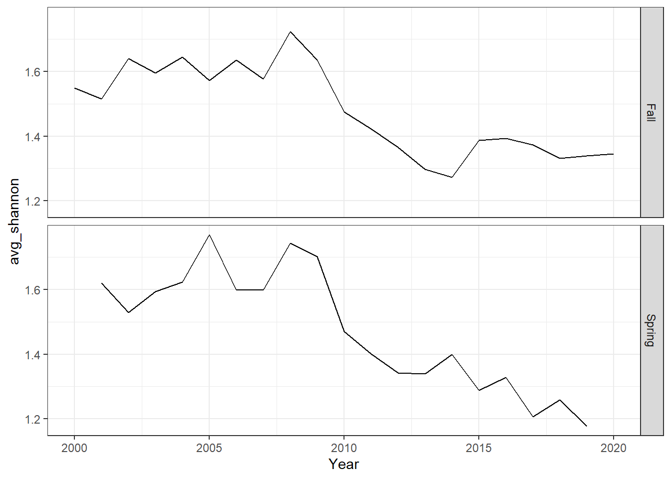

shannon<-group_by(data, Year,Tow_Number,COMMON_NAME)%>%
  mutate(species_total=sum(Expanded_Weight_kg, na.rm=TRUE))%>%
  group_by(Year, Tow_Number)%>%
  mutate(total=sum(species_total),prop=(species_total/total))%>%
  summarise(shannon=-1*(sum(prop*log(prop),na.rm=TRUE)))%>%
  group_by(Year)%>%
  summarise(avg_shannon=mean(shannon))

diversity<-ggplot()+geom_line(data=subset(shannon,Year>2005 & Year <2020), aes(Year, avg_shannon))+theme_classic()+ ylab(expression(paste("Shannon-Weiner\nDiversity")))+theme(plot.margin = margin(10, 10, 10, 20))

diversity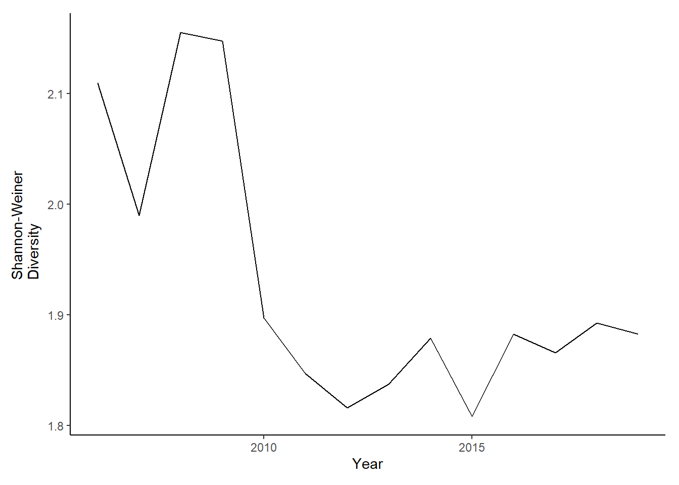

Simpson’s diversity and evenness

me_simpson<- group_by(data, Year, COMMON_NAME, Season, Tow_Number)%>%
  mutate(species_total=sum(Expanded_Weight_kg, na.rm=TRUE))%>%
  group_by(Year, Season, Tow_Number)%>%
  mutate(richness=length(unique(COMMON_NAME)))%>%
  mutate(total=sum(species_total))%>%
  mutate(prop=(species_total/total))%>%
  summarise(simpsonD=1/(sum(prop^2)), simpsonE=simpsonD*(1/richness))%>%
  group_by(Year, Season)%>%
  summarise(avg_simpsonD=mean(simpsonD), avg_simpsonE=mean(simpsonE))
# this code is not working properly, very high simpson's d and e??

ggplot()+geom_line(data=me_simpson, aes(Year, avg_simpsonE))+
  facet_grid(rows=vars(Season))+theme_bw()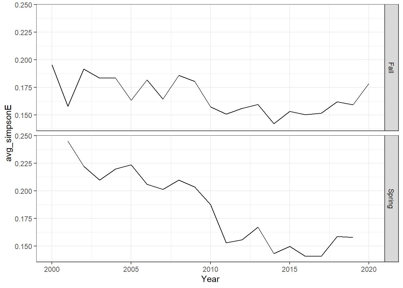

simpson<-group_by(data, Year,COMMON_NAME)%>%
  summarise(species_total=sum(Expanded_Weight_kg, na.rm=TRUE))%>% #aggregate to get yearly species totals
  group_by(Year)%>%
  mutate(richness=length(unique(COMMON_NAME)))%>%
  mutate(total=sum(species_total))%>%
  mutate(prop=(species_total/total))%>%
  summarise(simpsonD=1/(sum(prop^2)), simpsonE=simpsonD*(1/richness))%>%
  group_by(Year)%>%
  summarise(avg_simpsonD=mean(simpsonD), avg_simpsonE=mean(simpsonE))
   
ggplot()+geom_line(data=simpson, aes(Year, avg_simpsonD))+theme_classic()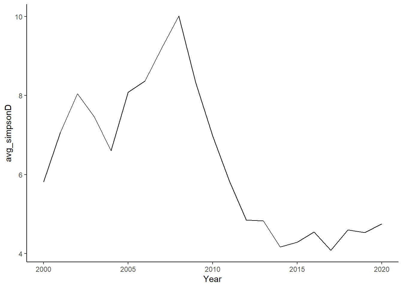

evenness<-ggplot()+geom_line(data=subset(simpson,Year>2005 & Year <2020), aes(Year, avg_simpsonE))+theme_classic()+ ylab(expression(paste("Simpson's\nEvenness")))+theme(plot.margin = margin(10, 10, 10, 20))

evenness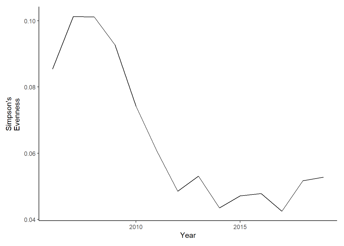

Average taxinomic distinctness

library(taxize)
library(purrr)
library(mgcv)

# data2<-read.csv(here("Data/common_scientific_convert.csv"))%>%
#   distinct(COMMON_NAME, .keep_all=TRUE)
# 
# data2<-left_join(data,data2, by="COMMON_NAME")

species <- filter(data,!is.na(SCIENTIFIC_NAME))%>%
  rename(Species=SCIENTIFIC_NAME)
  #add scientific name for taxonomic distinctness

#na<-filter(data, is.na(SCIENTIFIC_NAME))%>%
#  distinct(COMMON_NAME)

diff_species<-as.vector(unique(species$Species))
tax <- classification(diff_species, db = 'itis') 

## ==  142 queries  =============
## v  Found:  Alosa pseudoharengus
## v  Found:  Squalus acanthias
## v  Found:  Glyptocephalus cynoglossus
## v  Found:  Paralichthys oblongus
## v  Found:  Pseudopleuronectes americanus
## v  Found:  Limanda ferruginea
## v  Found:  Melanogrammus aeglefinus
## v  Found:  Urophycis chuss
## v  Found:  Merluccius bilinearis
## v  Found:  Urophycis tenuis
## v  Found:  Homarus americanus
## v  Found:  Lophius americanus
## v  Found:  Hippoglossoides platessoides
## v  Found:  Pollachius virens
## v  Found:  Zoarces americanus
## v  Found:  Myoxocephalus octodecemspinosus
## v  Found:  Centropristis striata
## v  Found:  Leucoraja erinacea
## v  Found:  Leucoraja ocellata
## v  Found:  Loligo pealeii
## v  Found:  Gadus morhua
## v  Found:  Cancer irroratus
## v  Found:  Enchelyopus cimbrius
## v  Found:  Placopecten magellanicus
## v  Found:  Prionotus carolinus
## v  Found:  Aspidophoroides monopterygius
## v  Found:  Cancer borealis
## v  Found:  Trachurus lathami
## v  Found:  Hemitripterus americanus
## v  Found:  Illex illecebrosus
## v  Found:  Peprilus triacanthus
## v  Found:  Tautogolabrus adspersus
## v  Found:  Clupea harengus
## v  Found:  Stenotomus chrysops
## v  Found:  Amblyraja radiata
## v  Found:  Sebastes fasciatus
## v  Found:  Scomber scombrus
## v  Found:  Pandalus borealis
## v  Found:  Alosa sapidissima
## v  Found:  Dichelopandalus leptocerus
## v  Found:  Brevoortia tyrannus
## v  Found:  Osmerus mordax
## v  Found:  Cryptacanthodes maculatus
## v  Found:  Menidia menidia
## v  Found:  Ammodytes americanus
## v  Found:  Acipenser oxyrinchus
## v  Found:  Cyclopterus lumpus
## v  Found:  Pandalus montagui
## v  Found:  Arctica islandica
## v  Found:  Caudina arenata
## v  Found:  Crangon septemspinosa
## v  Found:  Engraulis eurystole
## v  Found:  Chionoecetes opilio
## v  Found:  Cucumaria frondosa
## v  Found:  Urophycis regia
## v  Found:  Myoxocephalus scorpius
## v  Found:  Astarte undata
## v  Found:  Hyas araneus
## v  Found:  Lebbeus groenlandicus
## v  Found:  Triglops murrayi
## v  Found:  Citharichthys arctifrons
## v  Found:  Malacoraja senta
## v  Found:  Pitar morrhuanus
## v  Found:  Hippoglossus hippoglossus
## v  Found:  Carcinus maenas
## v  Found:  Cyclocardia borealis
## v  Found:  Chlamys islandica
## v  Found:  Strongylocentrotus droebachiensis
## v  Found:  Modiolus modiolus
## v  Found:  Zenopsis conchifera
## v  Found:  Decapterus punctatus
## v  Found:  Asterias vulgaris
## v  Found:  Maurolicus muelleri
## v  Found:  Torpedo nobiliana
## v  Found:  Lumpenus lumpretaeformis
## v  Found:  Lumpenus maculatus
## v  Found:  Gasterosteus aculeatus
## v  Found:  Reinhardtius hippoglossoides
## v  Found:  Anguilla rostrata
## v  Found:  Selene setapinnis
## v  Found:  Alosa aestivalis
## v  Found:  Syngnathus fuscus
## v  Found:  Pomatomus saltatrix
## v  Found:  Pristigenys alta
## v  Found:  Mytilus edulis
## v  Found:  Lithodes maja
## v  Found:  Peristedion miniatum
## v  Found:  Ulvaria subbifurcata
## v  Found:  Nemichthys scolopaceus
## v  Found:  Chaceon quinquedens
## v  Found:  Mercenaria mercenaria
## v  Found:  Pasiphaea multidentata
## v  Found:  Liparis coheni
## v  Found:  Dipturus laevis
## v  Found:  Lunatia heros
## v  Found:  Selar crumenophthalmus
## v  Found:  Liparis atlanticus
## v  Found:  Myxine glutinosa
## v  Found:  Lebbeus polaris
## v  Found:  Eualus fabricii
## v  Found:  Pandalus propinquus
## v  Found:  Liparis inquilinus
## v  Found:  Liparis liparis
## v  Found:  Neptunea decemcostata
## v  Found:  Anarhichas lupus
## v  Found:  Mallotus villosus
## v  Found:  Microgadus tomcod
## v  Found:  Pontophilus norvegicus
## v  Found:  Morone saxatilis
## v  Found:  Buccinum undatum
## v  Found:  Anchoa hepsetus
## v  Found:  Axius serratus
## v  Found:  Pholis gunnellus
## v  Found:  Raja eglanteria
## v  Found:  Decapterus macarellus
## v  Found:  Scomberesox saurus
## v  Found:  Lycenchelys verrilli
## v  Found:  Myoxocephalus aenaeus
## v  Found:  Liparis fabricii
## v  Found:  Monacanthus hispidus
## v  Found:  Spirontocaris liljeborgii
## v  Found:  Sphoeroides maculatus
## v  Found:  Melanostigma atlanticum
## v  Found:  Polymixia lowei
## v  Found:  Xenolepidichthys dalgleishi
## v  Found:  Spirontocaris spinus
## v  Found:  Colus stimpsoni
## v  Found:  Liparis tunicatus
## v  Found:  Phycis chesteri
## v  Found:  Helicolenus dactylopterus
## v  Found:  Ariomma bondi
## v  Found:  Lepophidium profundorum
## v  Found:  Lophius gastrophysus
## v  Found:  Ostrea edulis
## v  Found:  Menticirrhus saxatilis
## v  Found:  Antigonia combatia
## v  Found:  Brosme brosme
## v  Found:  Apeltes quadracus
## v  Found:  Sclerocrangon boreas
## v  Found:  Eumicrotremus spinosus
## v  Found:  Leucoraja garmani
## v  Found:  Ensis directus
## ==  Results  =================
## 
## * Total: 142 
## * Found: 142 
## * Not Found: 0

info <- matrix(NA)
expand <- matrix(NA)
specific <- matrix(NA, nrow = length(diff_species), ncol=6)


for (i in 1:length(tax)){
info <- tax[[i]][c('name','rank')]
expand <- info[info$rank == 'phylum'| info$rank == 'class'| info$rank == 'order' | info$rank == 'family' | info$rank == 'genus' | info$rank == 'species',]
specific[i,] <- as.vector(expand$name)

}
colnames(specific) <- c("Phylum", "Class", "Order", "Family", "Genus", "Species")
phylo<-as.data.frame(specific)

merge<-left_join(species,phylo, by="Species")
  
data_tax<-merge%>%
  filter(!is.na(Species))

data_tax_groups<-group_by(data_tax, Year, Season, Tow_Number, Species)%>%
  summarise(catch=sum(Expanded_Weight_kg, na.rm=TRUE))%>%
  mutate(indicator=cur_group_id())%>%
  left_join(phylo)

hauls <- unique(data_tax_groups$indicator)   
N_hauls <- length(hauls) # number of hauls
N_species <- NULL #N species
sub_species <- NULL # N_species-1
total <- NULL  #xixj
numerator <- NULL #wijxixj
x_y <- matrix(NA, nrow = 6, ncol = 6) 
x <- NULL
y <- NULL
ident <- NULL
weight <- NULL #wij
count <- NULL
total_weight <- NULL
mean_weight <- NULL
weight_var <- NULL
delta <- NULL
delta_star <- NULL
delta_plus <- NULL
delta_var <- NULL
weight_var <- NULL

for (j in 1:N_hauls) {  
diff_hauls <- data_tax_groups[which(data_tax_groups$indicator == j),] #subset unique hauls/functional groups
N_species[j] <- length(unique(diff_hauls$Species))# count the number of unique species in each haul (denominator)
sub_species[j] <- N_species[j]-1
diff <- unique(as.vector(diff_hauls$Species)) # name of each unique species 
combos <- combn(diff, 2) # create combinations of each species/haul (for weight calc)

phylo <- as.matrix(subset(diff_hauls, select = c(Phylum,Class,Order,Family,Genus, Species))) # extract phylogenetic information only
unique_phylo <- uniquecombs(phylo) # subset by unique species information
unique_phylo <- as.data.frame(unique_phylo)

total <- NULL  # reset the length for each haul because they will be different
weight <- NULL # reset  

for (i in 1:ncol(combos)) { # for each unique combination count the number of each species 
  total[i] <- sum(diff_hauls$Species == combos[1,i]) * sum(diff_hauls$Species == combos[2,i]) #empty vector is always length 210
  #total[i] <- diff_hauls[diff_hauls[,22] == combos[1,i],9] * diff_hauls[diff_hauls[,22] == combos[2,i],9]
  x <- unique_phylo[unique_phylo$Species == combos[1,i],]
  y <- unique_phylo[unique_phylo$Species == combos[2,i],]
  x_y <- rbind(x,y)
  
  for (k in 1:ncol(x_y)){ # for each combination calculate the weight value 
    ident[k] <- identical(as.vector(x_y[1,k]), as.vector(x_y[2,k])) # determine how much of phylogenetic information is the same
    weight[i] <- sum(ident == "FALSE") # vector of weights
    #mean_weight[i] <- mean(weight) #rep(mean(weight),length(weight))
    numerator[j] <- sum(total*weight) 
    count[j] <- sum(total)
    mean_weight[j] <- mean(weight)
    total_weight[j] <- sum(weight)
    weight_var[j] <- sum((weight- mean(weight))^2) 
  }
  delta <- (2*numerator)/(N_species*sub_species)
  delta_star <- numerator/(count)
  delta_plus <- (2*total_weight)/(N_species*sub_species)
  delta_var <- (2*weight_var)/(N_species*sub_species) #double check that this equation is correct
}
}
tow <- group_by(data,Year, Season, Tow_Number)%>%
  summarise()
tax_indices <- cbind(delta, delta_star, delta_plus, delta_var)
ind_by_haul <- cbind(tow, tax_indices)

# delta# taxonomic diversity
# delta_star # taxonomic distinctness
# delta_plus # average taxonomic distinctness
# delta_var # variation in taxonomic distinctness


d_season<-group_by(ind_by_haul,Year, Season)%>%
  summarise(avg_delta=mean(delta), avg_delta_star=mean(delta_star), avg_delta_plus=mean(delta_plus), avg_delta_var=mean(delta_var))

#write.csv(d, here("Data/tax_metrics.csv"))

tax.distinct_season<-ggplot()+geom_line(data=subset(d_season,Year>2005 & Year <2020), aes(Year, avg_delta_plus))+theme_bw()+ylab(expression(paste("Average\nTaxonomic\nDistinctness")))+theme(plot.margin = margin(10, 10, 10, 25))+ facet_grid(rows=vars(Season))
                                                                                     
tax.distinct_season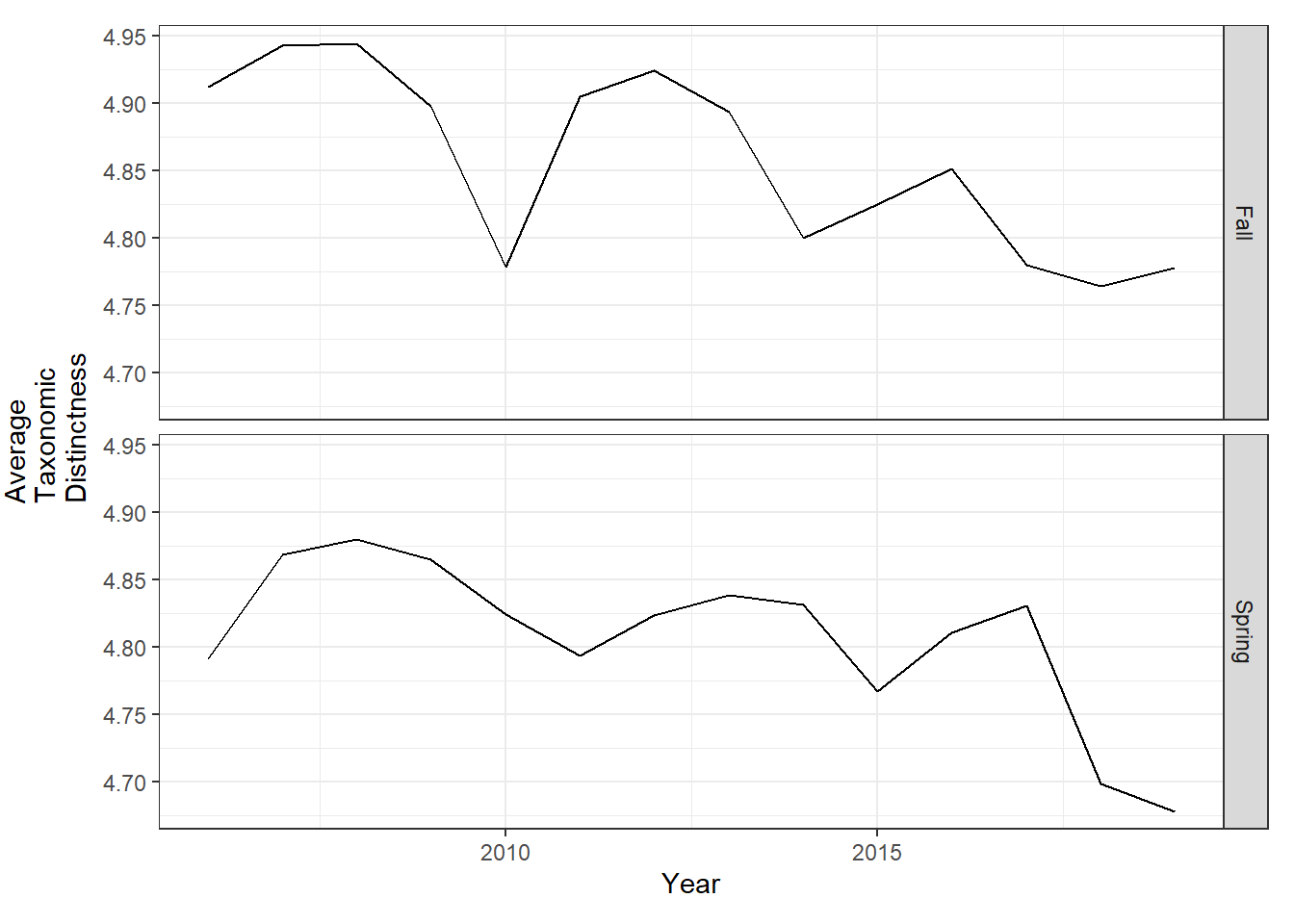

d<-group_by(ind_by_haul,Year)%>%
  summarise(avg_delta=mean(delta), avg_delta_star=mean(delta_star), avg_delta_plus=mean(delta_plus), avg_delta_var=mean(delta_var))

tax.distinct<-ggplot()+geom_line(data=subset(d,Year>2005 & Year <2020), aes(Year, avg_delta_plus))+theme_classic()+ylab(expression(paste("Average\nTaxonomic\nDistinctness")))+theme(plot.margin = margin(10, 10, 10, 25))

tax.distinct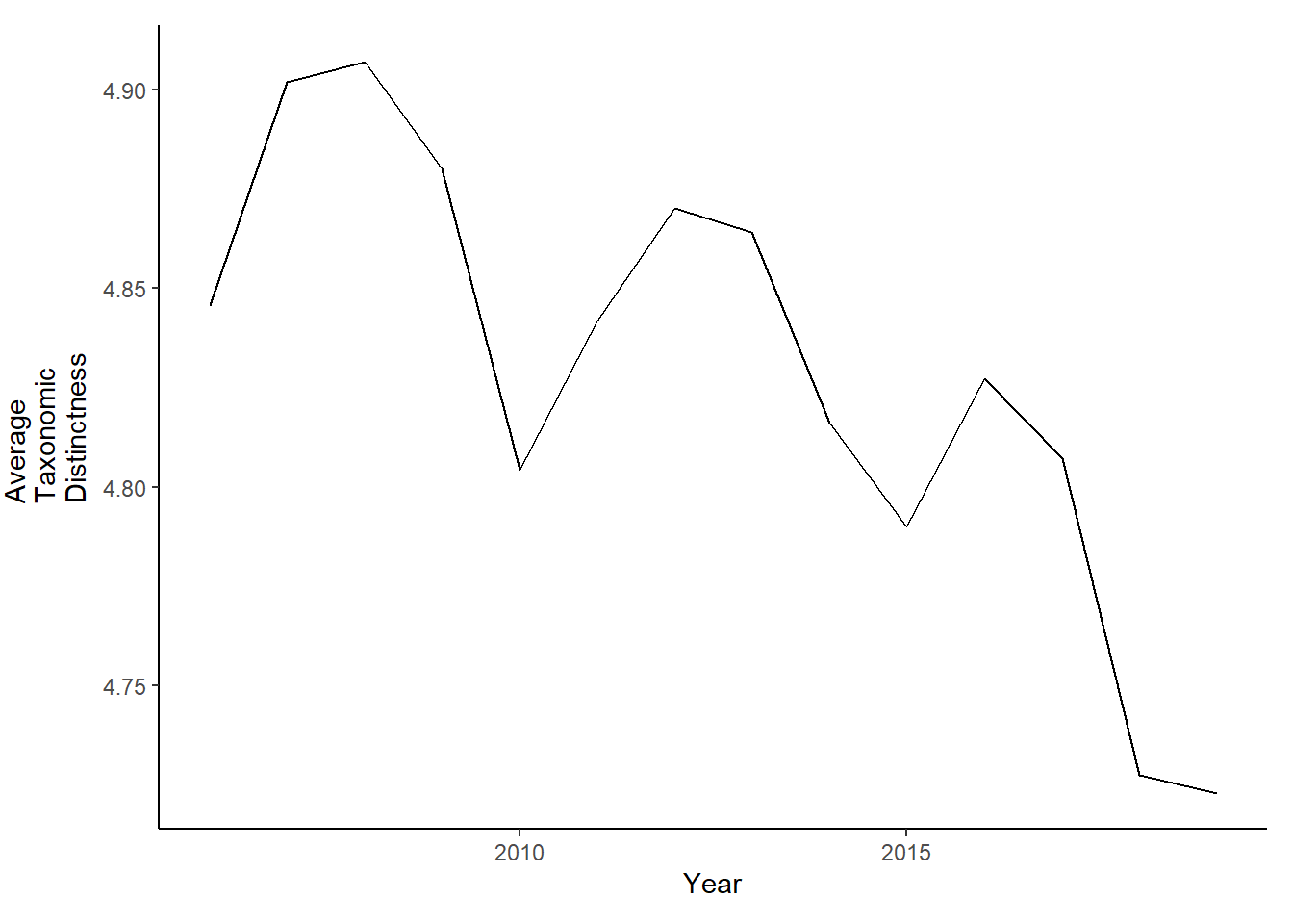

Combo plot

library(reshape2)
library(gridExtra)

all_metrics<-full_join(richness,shannon, by="Year")%>%
  full_join(simpson)%>%
  full_join(d)

#write.csv(all_metrics, here("Data/trawl_biodiversity_update.csv"))

all_melt<-melt(all_metrics, id="Year")

ggplot()+geom_line(data=all_melt, aes(Year,value))+facet_grid(rows = vars(variable), scales="free")+theme_bw()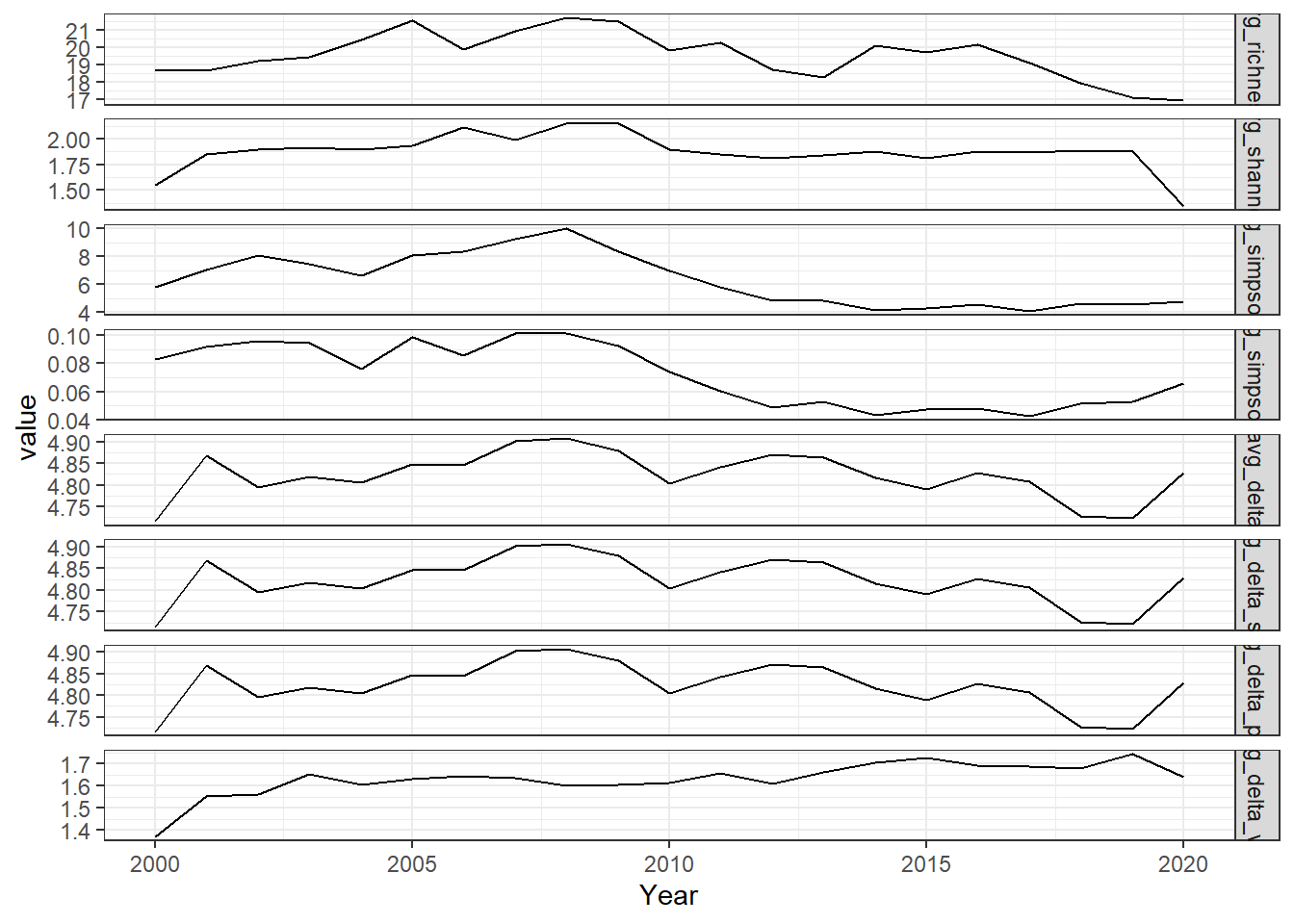

grid.arrange(rich, diversity, evenness,tax.distinct, nrow=4)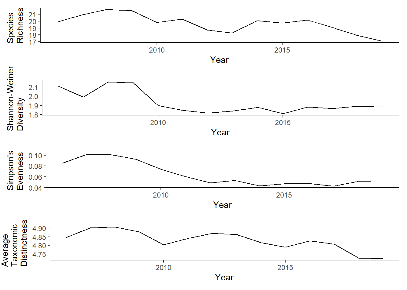

Regional diversity

data_regions<-data
# group to east/west of Penobscot Bay
data_regions$group<-NULL
data_regions$group[data_regions$Region==1]<-"East"
data_regions$group[data_regions$Region==2]<-"East"
data_regions$group[data_regions$Region==3]<-"Penobscot"
data_regions$group[data_regions$Region==4]<-"West"
data_regions$group[data_regions$Region==5]<-"West"

data_regions<-filter(data_regions,!is.na(group))%>%
  filter(Expanded_Weight_kg!=0)

Species richness

richness<-group_by(data_regions, group, Year, Tow_Number)%>%
  summarise(richness=length(unique(SCIENTIFIC_NAME)))%>%
  group_by(Year, group)%>%
  summarise(avg_richness=mean(richness, na.rm=TRUE))

ggplot()+ geom_line(data=richness, aes(Year, avg_richness))+
  facet_grid(rows=vars(group))+theme_bw()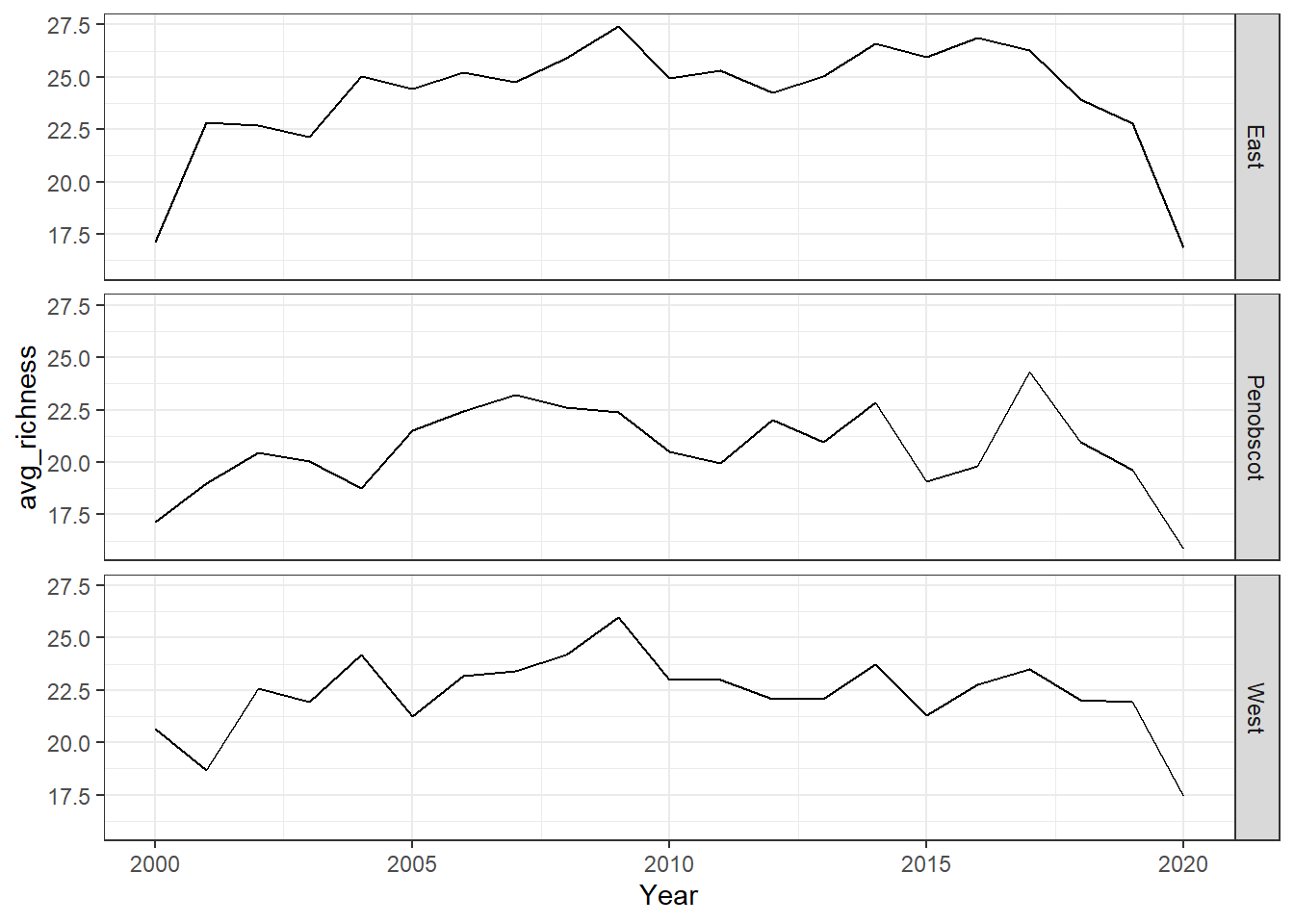

Shannon-Weiner diversity

shannon<-group_by(data_regions, Year,group, Tow_Number)%>%
  mutate(total=sum(Expanded_Weight_kg, na.rm=TRUE), prop=(Expanded_Weight_kg/total))%>%
  summarise(shannon=-1*(sum(prop*log(prop))))%>%
  group_by(Year, group)%>%
  summarise(avg_shannon=mean(shannon, na.rm=TRUE))

ggplot()+geom_line(data=shannon, aes(Year, avg_shannon))+
  facet_grid(rows=vars(group))+theme_bw()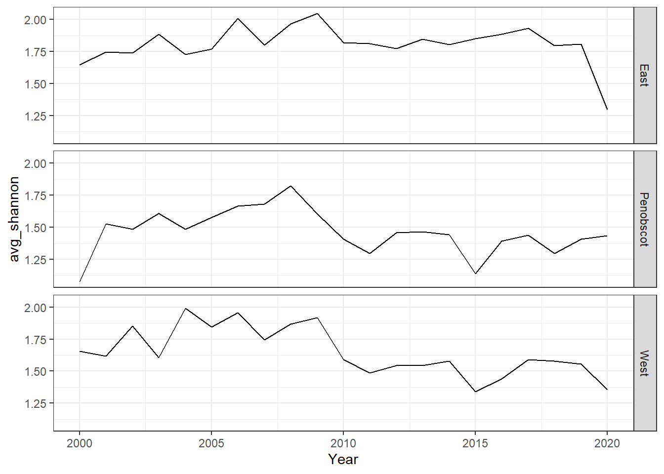

Simpson’s diversity and evenness

simpson<-group_by(data_regions, Year,group, Tow_Number,SCIENTIFIC_NAME)%>%
  summarise(species_total=sum(Expanded_Weight_kg, na.rm=TRUE))%>% #aggregate 
  group_by(Year, group, Tow_Number)%>%
  mutate(richness=length(unique(SCIENTIFIC_NAME)))%>%
  mutate(total=sum(species_total))%>%
  mutate(prop=species_total/total)%>%
  summarise(simpsonD=1/(sum(prop^2)),simpsonE=simpsonD*(1/richness))%>%
  group_by(Year, group)%>%
  summarise(avg_simpsonE=mean(simpsonE, na.rm=TRUE))

ggplot()+geom_line(data=simpson, aes(Year, avg_simpsonE))+
  facet_grid(rows=vars(group))+theme_bw()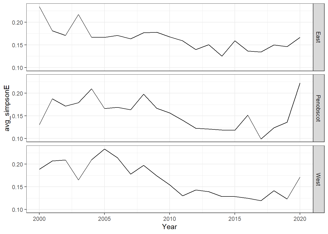

Average taxinomic distinctness

library(taxize)
library(purrr)
library(mgcv)
library(gridExtra)

species <- filter(data_regions,!is.na(SCIENTIFIC_NAME))%>%
  rename(Species=SCIENTIFIC_NAME)
  

diff_species<-as.vector(unique(species$Species))
tax <- classification(diff_species, db = 'itis') 

## ==  142 queries  =============
## v  Found:  Alosa pseudoharengus
## v  Found:  Squalus acanthias
## v  Found:  Glyptocephalus cynoglossus
## v  Found:  Paralichthys oblongus
## v  Found:  Pseudopleuronectes americanus
## v  Found:  Limanda ferruginea
## v  Found:  Melanogrammus aeglefinus
## v  Found:  Urophycis chuss
## v  Found:  Merluccius bilinearis
## v  Found:  Urophycis tenuis
## v  Found:  Homarus americanus
## v  Found:  Lophius americanus
## v  Found:  Hippoglossoides platessoides
## v  Found:  Pollachius virens
## v  Found:  Zoarces americanus
## v  Found:  Myoxocephalus octodecemspinosus
## v  Found:  Centropristis striata
## v  Found:  Leucoraja erinacea
## v  Found:  Leucoraja ocellata
## v  Found:  Loligo pealeii
## v  Found:  Gadus morhua
## v  Found:  Cancer irroratus
## v  Found:  Enchelyopus cimbrius
## v  Found:  Placopecten magellanicus
## v  Found:  Prionotus carolinus
## v  Found:  Aspidophoroides monopterygius
## v  Found:  Cancer borealis
## v  Found:  Trachurus lathami
## v  Found:  Hemitripterus americanus
## v  Found:  Illex illecebrosus
## v  Found:  Peprilus triacanthus
## v  Found:  Tautogolabrus adspersus
## v  Found:  Clupea harengus
## v  Found:  Stenotomus chrysops
## v  Found:  Amblyraja radiata
## v  Found:  Sebastes fasciatus
## v  Found:  Scomber scombrus
## v  Found:  Pandalus borealis
## v  Found:  Alosa sapidissima
## v  Found:  Dichelopandalus leptocerus
## v  Found:  Brevoortia tyrannus
## v  Found:  Osmerus mordax
## v  Found:  Cryptacanthodes maculatus
## v  Found:  Menidia menidia
## v  Found:  Ammodytes americanus
## v  Found:  Acipenser oxyrinchus
## v  Found:  Cyclopterus lumpus
## v  Found:  Pandalus montagui
## v  Found:  Arctica islandica
## v  Found:  Caudina arenata
## v  Found:  Crangon septemspinosa
## v  Found:  Engraulis eurystole
## v  Found:  Chionoecetes opilio
## v  Found:  Cucumaria frondosa
## v  Found:  Urophycis regia
## v  Found:  Myoxocephalus scorpius
## v  Found:  Astarte undata
## v  Found:  Hyas araneus
## v  Found:  Lebbeus groenlandicus
## v  Found:  Triglops murrayi
## v  Found:  Citharichthys arctifrons
## v  Found:  Malacoraja senta
## v  Found:  Pitar morrhuanus
## v  Found:  Hippoglossus hippoglossus
## v  Found:  Carcinus maenas
## v  Found:  Cyclocardia borealis
## v  Found:  Chlamys islandica
## v  Found:  Strongylocentrotus droebachiensis
## v  Found:  Modiolus modiolus
## v  Found:  Zenopsis conchifera
## v  Found:  Decapterus punctatus
## v  Found:  Asterias vulgaris
## v  Found:  Maurolicus muelleri
## v  Found:  Torpedo nobiliana
## v  Found:  Lumpenus lumpretaeformis
## v  Found:  Lumpenus maculatus
## v  Found:  Gasterosteus aculeatus
## v  Found:  Reinhardtius hippoglossoides
## v  Found:  Anguilla rostrata
## v  Found:  Selene setapinnis
## v  Found:  Alosa aestivalis
## v  Found:  Syngnathus fuscus
## v  Found:  Pomatomus saltatrix
## v  Found:  Pristigenys alta
## v  Found:  Mytilus edulis
## v  Found:  Lithodes maja
## v  Found:  Peristedion miniatum
## v  Found:  Ulvaria subbifurcata
## v  Found:  Nemichthys scolopaceus
## v  Found:  Chaceon quinquedens
## v  Found:  Mercenaria mercenaria
## v  Found:  Pasiphaea multidentata
## v  Found:  Liparis coheni
## v  Found:  Dipturus laevis
## v  Found:  Lunatia heros
## v  Found:  Selar crumenophthalmus
## v  Found:  Liparis atlanticus
## v  Found:  Myxine glutinosa
## v  Found:  Lebbeus polaris
## v  Found:  Eualus fabricii
## v  Found:  Pandalus propinquus
## v  Found:  Liparis inquilinus
## v  Found:  Liparis liparis
## v  Found:  Neptunea decemcostata
## v  Found:  Anarhichas lupus
## v  Found:  Mallotus villosus
## v  Found:  Microgadus tomcod
## v  Found:  Pontophilus norvegicus
## v  Found:  Morone saxatilis
## v  Found:  Buccinum undatum
## v  Found:  Anchoa hepsetus
## v  Found:  Axius serratus
## v  Found:  Pholis gunnellus
## v  Found:  Raja eglanteria
## v  Found:  Decapterus macarellus
## v  Found:  Scomberesox saurus
## v  Found:  Lycenchelys verrilli
## v  Found:  Myoxocephalus aenaeus
## v  Found:  Liparis fabricii
## v  Found:  Monacanthus hispidus
## v  Found:  Spirontocaris liljeborgii
## v  Found:  Sphoeroides maculatus
## v  Found:  Melanostigma atlanticum
## v  Found:  Polymixia lowei
## v  Found:  Xenolepidichthys dalgleishi
## v  Found:  Spirontocaris spinus
## v  Found:  Colus stimpsoni
## v  Found:  Liparis tunicatus
## v  Found:  Phycis chesteri
## v  Found:  Helicolenus dactylopterus
## v  Found:  Ariomma bondi
## v  Found:  Lepophidium profundorum
## v  Found:  Lophius gastrophysus
## v  Found:  Ostrea edulis
## v  Found:  Menticirrhus saxatilis
## v  Found:  Antigonia combatia
## v  Found:  Brosme brosme
## v  Found:  Apeltes quadracus
## v  Found:  Sclerocrangon boreas
## v  Found:  Eumicrotremus spinosus
## v  Found:  Leucoraja garmani
## v  Found:  Ensis directus
## ==  Results  =================
## 
## * Total: 142 
## * Found: 142 
## * Not Found: 0

info <- matrix(NA)
expand <- matrix(NA)
specific <- matrix(NA, nrow = length(diff_species), ncol=6)


for (i in 1:length(tax)){
info <- tax[[i]][c('name','rank')]
expand <- info[info$rank == 'phylum'| info$rank == 'class'| info$rank == 'order' | info$rank == 'family' | info$rank == 'genus' | info$rank == 'species',]
specific[i,] <- as.vector(expand$name)

}
colnames(specific) <- c("Phylum", "Class", "Order", "Family", "Genus", "Species")
phylo<-as.data.frame(specific)

merge<-left_join(species,phylo, by="Species")
  
landings_tax<-rename(data_regions, Species=SCIENTIFIC_NAME)


#break into groups
east_species<-filter(landings_tax, group=="East")%>%
  group_by(Year,group,Season,Tow_Number,Species)%>%
  summarise(weight=sum(weight))%>%
  mutate(indicator=cur_group_id())%>%
  left_join(phylo)
  
west_species<-filter(landings_tax, group=="West")%>%
  group_by(Year,group,Season, Tow_Number,Species)%>%
  summarise(weight=sum(weight))%>%
  mutate(indicator=cur_group_id())%>%
  left_join(phylo)

pen_species<-filter(landings_tax, group=="Penobscot")%>%
  group_by(Year,group,Season,Tow_Number,Species)%>%
  summarise(weight=sum(weight))%>%
  mutate(indicator=cur_group_id())%>%
  left_join(phylo)

#east
hauls <- unique(east_species$indicator)   
N_hauls <- length(hauls) # number of hauls
N_species <- NULL #N species
sub_species <- NULL # N_species-1
total <- NULL  #xixj
numerator <- NULL #wijxixj
x_y <- matrix(NA, nrow = 6, ncol = 6) 
x <- NULL
y <- NULL
ident <- NULL
weight <- NULL #wij
count <- NULL
total_weight <- NULL
mean_weight <- NULL
weight_var <- NULL
delta <- NULL
delta_star <- NULL
delta_plus <- NULL
delta_var <- NULL
weight_var <- NULL

for (j in 1:N_hauls) {  
diff_hauls <- east_species[which(east_species$indicator == j),] #subset unique hauls/functional groups
N_species[j] <- length(unique(diff_hauls$Species))# count the number of unique species in each haul (denominator)
sub_species[j] <- N_species[j]-1
diff <- unique(as.vector(diff_hauls$Species)) # name of each unique species 
combos <- combn(diff, 2) # create combinations of each species/haul (for weight calc)

phylo <- as.matrix(subset(diff_hauls, select = c(Phylum,Class,Order,Family,Genus, Species))) # extract phylogenetic information only
unique_phylo <- uniquecombs(phylo) # subset by unique species information
unique_phylo <- as.data.frame(unique_phylo)

total <- NULL  # reset the length for each haul because they will be different
weight <- NULL # reset  

for (i in 1:ncol(combos)) { # for each unique combination count the number of each species 
  total[i] <- sum(diff_hauls$Species == combos[1,i]) * sum(diff_hauls$Species == combos[2,i]) #empty vector is always length 210
  #total[i] <- diff_hauls[diff_hauls[,22] == combos[1,i],9] * diff_hauls[diff_hauls[,22] == combos[2,i],9]
  x <- unique_phylo[unique_phylo$Species == combos[1,i],]
  y <- unique_phylo[unique_phylo$Species == combos[2,i],]
  x_y <- rbind(x,y)
  
  for (k in 1:ncol(x_y)){ # for each combination calculate the weight value 
    ident[k] <- identical(as.vector(x_y[1,k]), as.vector(x_y[2,k])) # determine how much of phylogenetic information is the same
    weight[i] <- sum(ident == "FALSE") # vector of weights
    #mean_weight[i] <- mean(weight) #rep(mean(weight),length(weight))
    numerator[j] <- sum(total*weight) 
    count[j] <- sum(total)
    mean_weight[j] <- mean(weight)
    total_weight[j] <- sum(weight)
    weight_var[j] <- sum((weight- mean(weight))^2) 
  }
  delta <- (2*numerator)/(N_species*sub_species)
  delta_star <- numerator/(count)
  delta_plus <- (2*total_weight)/(N_species*sub_species)
  delta_var <- (2*weight_var)/(N_species*sub_species) #double check that this equation is correct
}
}

tow <- group_by(east_species,Year, Season, Tow_Number)%>%
  summarise()
tax_indices <- cbind(delta, delta_star, delta_plus, delta_var)
ind_by_haul <- cbind(tow, tax_indices)

east_d<-group_by(ind_by_haul,Year, Season)%>%
  summarise(avg_delta=mean(delta, na.rm=TRUE), avg_delta_star=mean(delta_star, na.rm=TRUE), avg_delta_plus=mean(delta_plus, na.rm=TRUE), avg_delta_var=mean(delta_var, na.rm=TRUE))

#write.csv(d, here("Data/tax_metrics.csv"))

east_tax.distinct<-ggplot()+geom_line(data=subset(east_d, Year<2020), aes(Year, avg_delta_plus))+theme_classic()+ylab(expression(paste("East\nAverage\nTaxonomic\nDistinctness")))+theme(plot.margin = margin(10, 10, 10, 35))
                                                                        
#west
hauls <- unique(west_species$indicator)   
N_hauls <- length(hauls) # number of hauls
N_species <- NULL #N species
sub_species <- NULL # N_species-1
total <- NULL  #xixj
numerator <- NULL #wijxixj
x_y <- matrix(NA, nrow = 6, ncol = 6) 
x <- NULL
y <- NULL
ident <- NULL
weight <- NULL #wij
count <- NULL
total_weight <- NULL
mean_weight <- NULL
weight_var <- NULL
delta <- NULL
delta_star <- NULL
delta_plus <- NULL
delta_var <- NULL
weight_var <- NULL

for (j in 1:N_hauls) {  
diff_hauls <- west_species[which(west_species$indicator == j),] #subset unique hauls/functional groups
N_species[j] <- length(unique(diff_hauls$Species))# count the number of unique species in each haul (denominator)
sub_species[j] <- N_species[j]-1
diff <- unique(as.vector(diff_hauls$Species)) # name of each unique species 
combos <- combn(diff, 2) # create combinations of each species/haul (for weight calc)

phylo <- as.matrix(subset(diff_hauls, select = c(Phylum,Class,Order,Family,Genus, Species))) # extract phylogenetic information only
unique_phylo <- uniquecombs(phylo) # subset by unique species information
unique_phylo <- as.data.frame(unique_phylo)

total <- NULL  # reset the length for each haul because they will be different
weight <- NULL # reset  

for (i in 1:ncol(combos)) { # for each unique combination count the number of each species 
  total[i] <- sum(diff_hauls$Species == combos[1,i]) * sum(diff_hauls$Species == combos[2,i]) #empty vector is always length 210
  #total[i] <- diff_hauls[diff_hauls[,22] == combos[1,i],9] * diff_hauls[diff_hauls[,22] == combos[2,i],9]
  x <- unique_phylo[unique_phylo$Species == combos[1,i],]
  y <- unique_phylo[unique_phylo$Species == combos[2,i],]
  x_y <- rbind(x,y)
  
  for (k in 1:ncol(x_y)){ # for each combination calculate the weight value 
    ident[k] <- identical(as.vector(x_y[1,k]), as.vector(x_y[2,k])) # determine how much of phylogenetic information is the same
    weight[i] <- sum(ident == "FALSE") # vector of weights
    #mean_weight[i] <- mean(weight) #rep(mean(weight),length(weight))
    numerator[j] <- sum(total*weight) 
    count[j] <- sum(total)
    mean_weight[j] <- mean(weight)
    total_weight[j] <- sum(weight)
    weight_var[j] <- sum((weight- mean(weight))^2) 
  }
  delta <- (2*numerator)/(N_species*sub_species)
  delta_star <- numerator/(count)
  delta_plus <- (2*total_weight)/(N_species*sub_species)
  delta_var <- (2*weight_var)/(N_species*sub_species) #double check that this equation is correct
}
}

tow <- group_by(west_species,Year, Season, Tow_Number)%>%
  summarise()
tax_indices <- cbind(delta, delta_star, delta_plus, delta_var)
ind_by_haul <- cbind(tow, tax_indices)

west_d<-group_by(ind_by_haul,Year, Season)%>%
  summarise(avg_delta=mean(delta, na.rm=TRUE), avg_delta_star=mean(delta_star, na.rm=TRUE), avg_delta_plus=mean(delta_plus, na.rm=TRUE), avg_delta_var=mean(delta_var, na.rm=TRUE))

#write.csv(d, here("Data/tax_metrics.csv"))

west_tax.distinct<-ggplot()+geom_line(data=subset(west_d, Year<2020), aes(Year, avg_delta_plus))+theme_classic()+ylab(expression(paste("West\nAverage\nTaxinomic\nDistinctness")))+theme(plot.margin = margin(10, 10, 10, 35))
                                                                         

#Penobscot
hauls <- unique(pen_species$indicator)   
N_hauls <- length(hauls) # number of hauls
N_species <- NULL #N species
sub_species <- NULL # N_species-1
total <- NULL  #xixj
numerator <- NULL #wijxixj
x_y <- matrix(NA, nrow = 6, ncol = 6) 
x <- NULL
y <- NULL
ident <- NULL
weight <- NULL #wij
count <- NULL
total_weight <- NULL
mean_weight <- NULL
weight_var <- NULL
delta <- NULL
delta_star <- NULL
delta_plus <- NULL
delta_var <- NULL
weight_var <- NULL

for (j in 1:N_hauls) {  
diff_hauls <- pen_species[which(pen_species$indicator == j),] #subset unique hauls/functional groups
N_species[j] <- length(unique(diff_hauls$Species))# count the number of unique species in each haul (denominator)
sub_species[j] <- N_species[j]-1
diff <- unique(as.vector(diff_hauls$Species)) # name of each unique species 
combos <- combn(diff, 2) # create combinations of each species/haul (for weight calc)

phylo <- as.matrix(subset(diff_hauls, select = c(Phylum,Class,Order,Family,Genus, Species))) # extract phylogenetic information only
unique_phylo <- uniquecombs(phylo) # subset by unique species information
unique_phylo <- as.data.frame(unique_phylo)

total <- NULL  # reset the length for each haul because they will be different
weight <- NULL # reset  

for (i in 1:ncol(combos)) { # for each unique combination count the number of each species 
  total[i] <- sum(diff_hauls$Species == combos[1,i]) * sum(diff_hauls$Species == combos[2,i]) #empty vector is always length 210
  #total[i] <- diff_hauls[diff_hauls[,22] == combos[1,i],9] * diff_hauls[diff_hauls[,22] == combos[2,i],9]
  x <- unique_phylo[unique_phylo$Species == combos[1,i],]
  y <- unique_phylo[unique_phylo$Species == combos[2,i],]
  x_y <- rbind(x,y)
  
  for (k in 1:ncol(x_y)){ # for each combination calculate the weight value 
    ident[k] <- identical(as.vector(x_y[1,k]), as.vector(x_y[2,k])) # determine how much of phylogenetic information is the same
    weight[i] <- sum(ident == "FALSE") # vector of weights
    #mean_weight[i] <- mean(weight) #rep(mean(weight),length(weight))
    numerator[j] <- sum(total*weight) 
    count[j] <- sum(total)
    mean_weight[j] <- mean(weight)
    total_weight[j] <- sum(weight)
    weight_var[j] <- sum((weight- mean(weight))^2) 
  }
  delta <- (2*numerator)/(N_species*sub_species)
  delta_star <- numerator/(count)
  delta_plus <- (2*total_weight)/(N_species*sub_species)
  delta_var <- (2*weight_var)/(N_species*sub_species) #double check that this equation is correct
}
}



tow <- group_by(pen_species,Year, Season, Tow_Number)%>%
  summarise()
tax_indices <- cbind(delta, delta_star, delta_plus, delta_var)
ind_by_haul <- cbind(tow, tax_indices)

pen_d<-group_by(ind_by_haul, Year, Season)%>%
  summarise(avg_delta=mean(delta, na.rm=TRUE), avg_delta_star=mean(delta_star, na.rm=TRUE), avg_delta_plus=mean(delta_plus, na.rm=TRUE), avg_delta_var=mean(delta_var, na.rm=TRUE))

#write.csv(d, here("Data/tax_metrics.csv"))

pen_tax.distinct<-ggplot()+geom_line(data=subset(pen_d, Year<2020), aes(Year, avg_delta_plus))+theme_classic()+ylab(expression(paste("Penobscot\nAverage\nTaxonomic\nDistinctness")))+theme(plot.margin = margin(10, 10, 10, 35))

grid.arrange(east_tax.distinct, west_tax.distinct, pen_tax.distinct, nrow=3)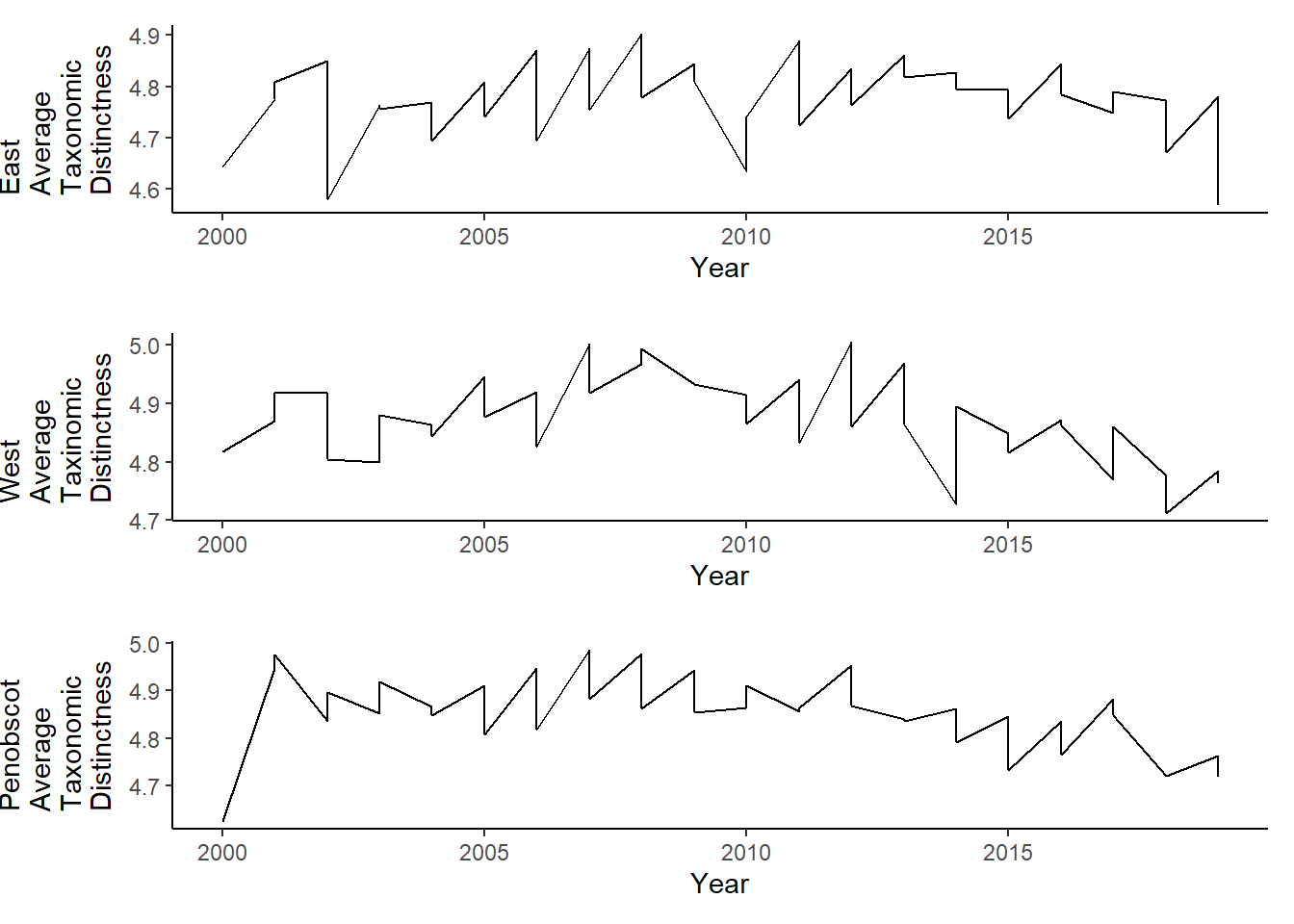                                                                        

East of Penobscot Bay

#combo plots

#east
r<-ggplot()+geom_line(data=subset(richness, group=="East" & Year<2020),aes(Year, avg_richness))+theme_classic()+ylab(expression(paste("Species\nRichness")))+theme(plot.margin = margin(10, 10, 10, 20))

s<-ggplot()+geom_line(data=subset(shannon, group=="East" & Year<2020),aes(Year, avg_shannon))+theme_classic()+ylab(expression(paste("Shannon-Weiner\nDiversity")))+theme(plot.margin = margin(10, 10, 10, 20))

e<-ggplot()+geom_line(data=subset(simpson, group=="East" & Year<2020),aes(Year, avg_simpsonE))+theme_classic()+ylab(expression(paste("Simpson's\nEvenness")))+theme(plot.margin = margin(10, 10, 10, 20))

t<-ggplot()+geom_line(data = subset(east_d, Year<2020), aes(Year, avg_delta_plus))+theme_classic()+ylab(expression(paste("Average\nTaxonomic\nDistinctness")))+theme(plot.margin = margin(10, 10, 10, 25))

grid.arrange(r,s,e,t, nrow=4)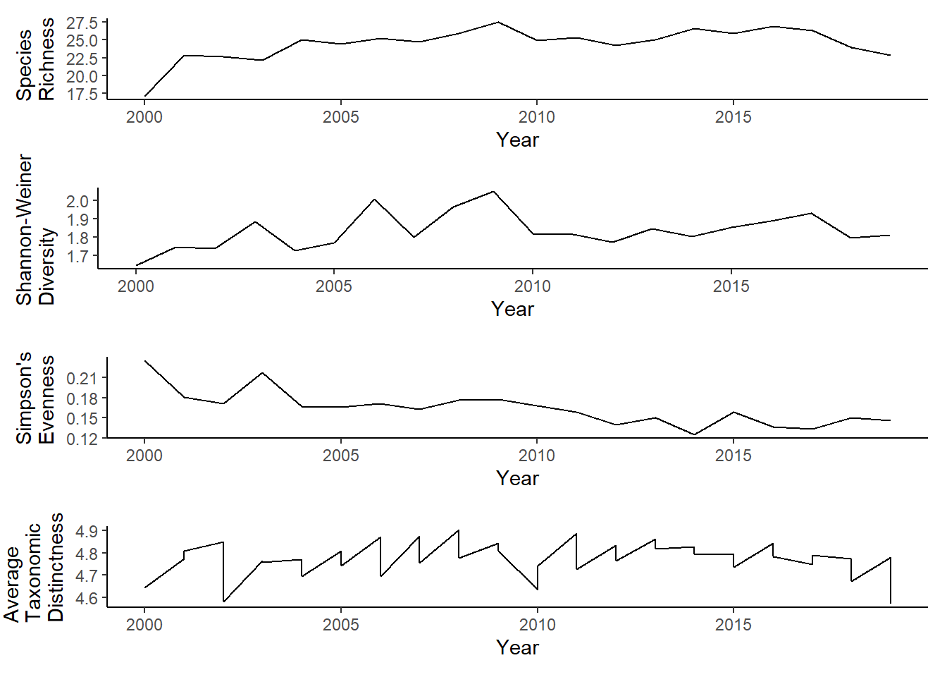

West of Penobscot Bay

#west
r<-ggplot()+geom_line(data=subset(richness, group=="West" & Year<2020),aes(Year, avg_richness))+theme_classic()+ylab(expression(paste("Species\nRichness")))+theme(plot.margin = margin(10, 10, 10, 20))

s<-ggplot()+geom_line(data=subset(shannon, group=="West" & Year<2020),aes(Year, avg_shannon))+theme_classic()+ylab(expression(paste("Shannon-Weiner\nDiversity")))+theme(plot.margin = margin(10, 10, 10, 20))

e<-ggplot()+geom_line(data=subset(simpson, group=="West" & Year<2020),aes(Year, avg_simpsonE))+theme_classic()+ ylab(expression(paste("Simpson's\nEvenness")))+theme(plot.margin = margin(10, 10, 10, 20))

t<-ggplot()+geom_line(data = subset(west_d, Year<2020), aes(Year, avg_delta_plus))+theme_classic()+ylab(expression(paste("Average\nTaxonomic\nDistinctness")))+theme(plot.margin = margin(10, 10, 10, 25))

grid.arrange(r,s,e,t, nrow=4)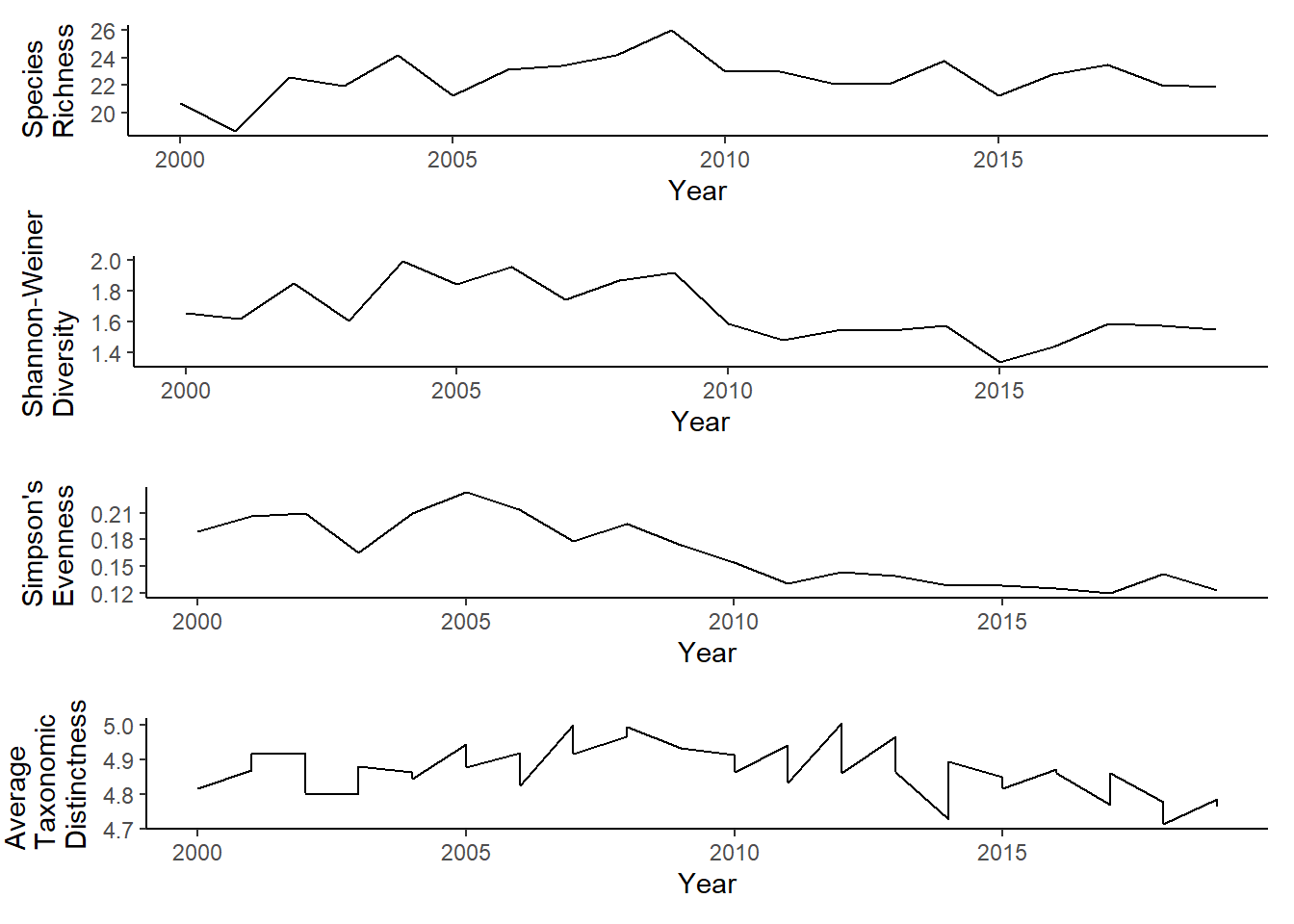

Penobscot Bay

#pen bay
r<-ggplot()+geom_line(data=subset(richness, group=="Penobscot" & Year<2020),aes(Year, avg_richness))+theme_classic()+ylab(expression(paste("Species\nRichness")))+theme(plot.margin = margin(10, 10, 10, 20))

s<-ggplot()+geom_line(data=subset(shannon, group=="Penobscot"& Year<2020),aes(Year, avg_shannon))+theme_classic()+ylab(expression(paste("Shannon-Weiner\nDiversity")))+theme(plot.margin = margin(10, 10, 10, 20))

e<-ggplot()+geom_line(data=subset(simpson, group=="Penobscot"& Year<2020),aes(Year, avg_simpsonE))+theme_classic()+ ylab(expression(paste("Simpson's\nEvenness")))+theme(plot.margin = margin(10, 10, 10, 20))

t<-ggplot()+geom_line(data = subset(pen_d, Year<2020), aes(Year, avg_delta_plus))+theme_classic()+ylab(expression(paste("Average\nTaxonomic\nDistinctness")))+theme(plot.margin = margin(10, 10, 10, 25))

grid.arrange(r,s,e,t, nrow=4)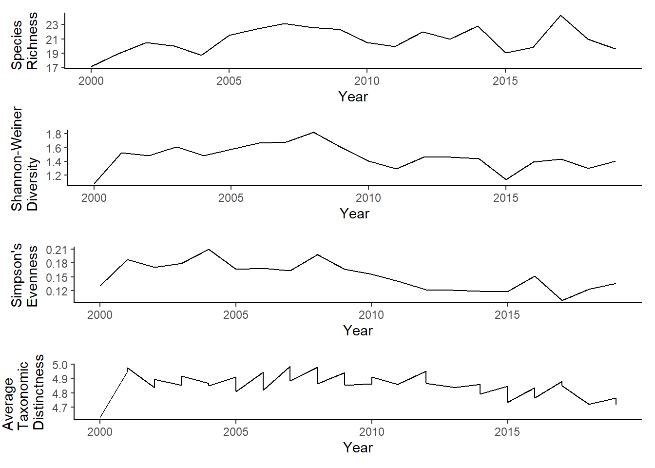

MA DMF Inshore Trawl Survey biodiversity metrics

setwd("C:/Users/jjesse/Box/Kerr Lab/Fisheries Science Lab/ME NH Trawl- Seagrant/Seagrant-AEW/MDMF")
ma_spring_inds <- read.csv("MDMF_spring_div_ind_by_tow.csv")%>%
  group_by(YEAR)%>%
  summarise(avg_N_species=mean(N_species), avg_H_index=mean(H_index), avg_D_index=mean(D_index), avg_E_index=mean(E_index), avg_delta=mean(delta), avg_delta_star=mean(delta_star), avg_delta_plus=mean(delta_plus), avg_delta_var=mean(delta_var))

ma_fall_inds <- read.csv("MDMF_fall_div_ind_by_tow.csv")%>%
  group_by(YEAR)%>%
  summarise(avg_N_species=mean(N_species, na.rm=TRUE), avg_H_index=mean(H_index, na.rm=TRUE), avg_D_index=mean(D_index, na.rm=TRUE), avg_E_index=mean(E_index, na.rm=TRUE), avg_delta=mean(delta, na.rm=TRUE), avg_delta_star=mean(delta_star, na.rm=TRUE), avg_delta_plus=mean(delta_plus, na.rm=TRUE), avg_delta_var=mean(delta_var, na.rm=TRUE))

Species richness

ma_sp_richness<-ggplot()+geom_line(data=ma_spring_inds, aes(YEAR, avg_N_species))+theme_classic()+ylab(expression(paste("Species\nRichness")))+theme(plot.margin = margin(10, 10, 10, 25))
                                   
ma_fl_richness<-ggplot()+geom_line(data=ma_fall_inds, aes(YEAR, avg_N_species))+theme_classic()+ylab(expression(paste("Species\nRichness")))+theme(plot.margin = margin(10, 10, 10, 25)) 

ma_sp_richness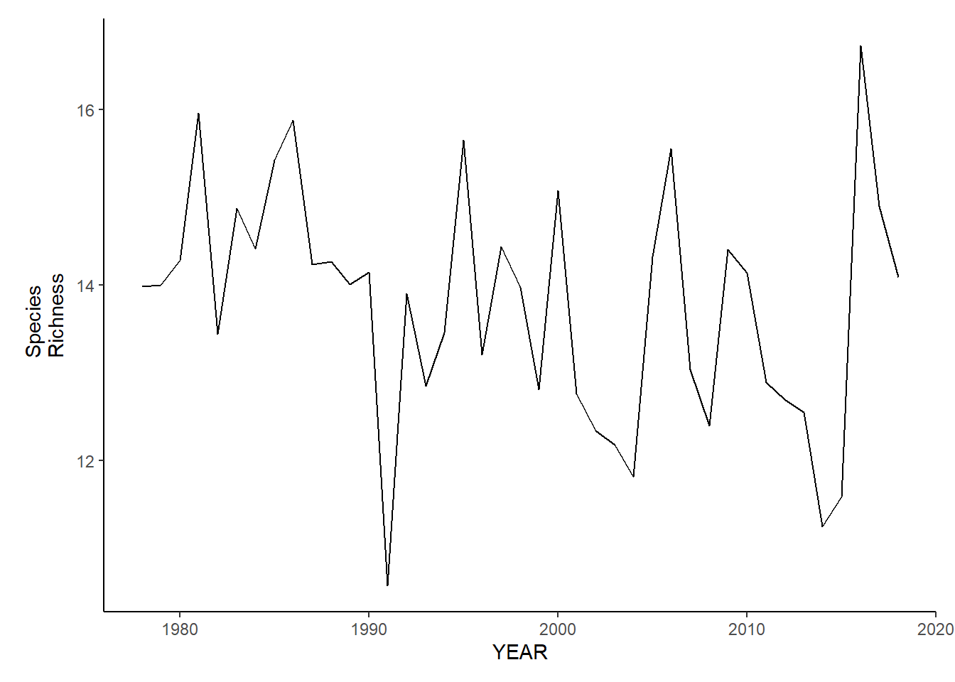

ma_fl_richness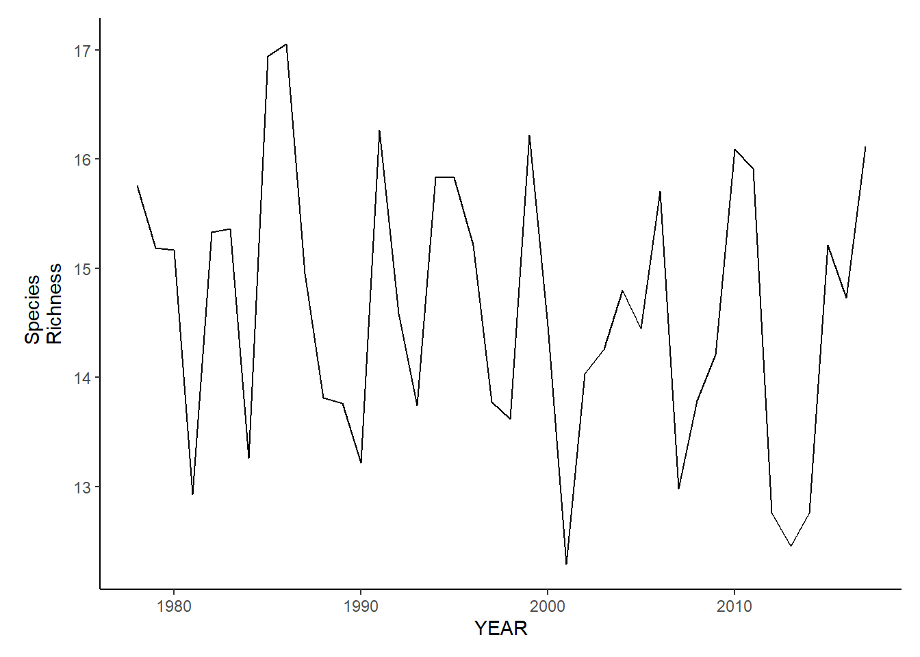

Shannon-Weiner diversity

ma_sp_shannon<-ggplot()+geom_line(data=ma_spring_inds, aes(YEAR, avg_H_index))+theme_classic()+ylab(expression(paste("Simpson's\nEvenness")))+theme(plot.margin = margin(10, 10, 10, 25))
                                   
ma_fl_shannon<-ggplot()+geom_line(data=ma_fall_inds, aes(YEAR, avg_H_index))+theme_classic()+ylab(expression(paste("Simpson's\nEvenness")))+theme(plot.margin = margin(10, 10, 10, 25)) 

ma_sp_shannon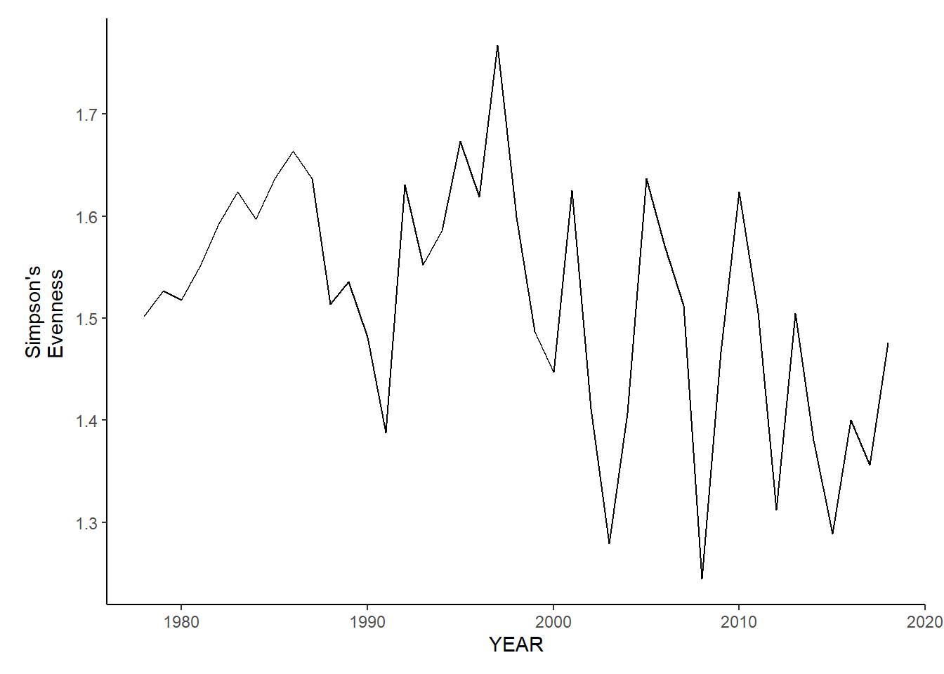

ma_fl_shannon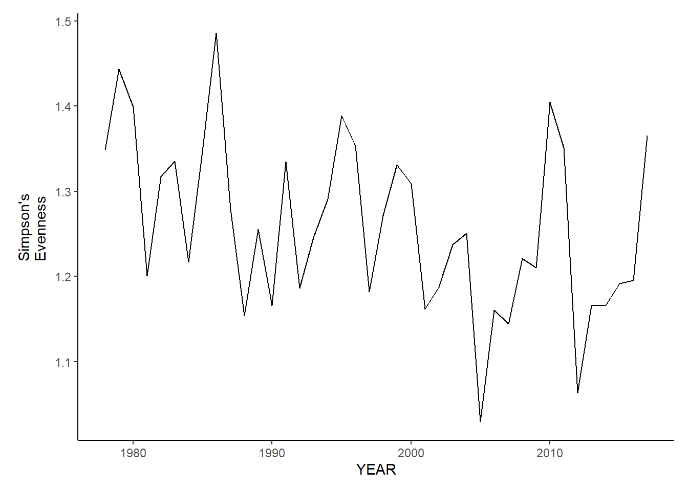

Simpson’s diversity

ma_sp_simpson.d<-ggplot()+geom_line(data=ma_spring_inds, aes(YEAR, avg_D_index))+theme_classic()+ylab(expression(paste("Simpson's\nDiversity")))+theme(plot.margin = margin(10, 10, 10, 25))
                                   
ma_fl_simpson.d<-ggplot()+geom_line(data=ma_fall_inds, aes(YEAR, avg_D_index))+theme_classic()+ylab(expression(paste("Simpson's\nDiversity")))+theme(plot.margin = margin(10, 10, 10, 25)) 

ma_sp_simpson.d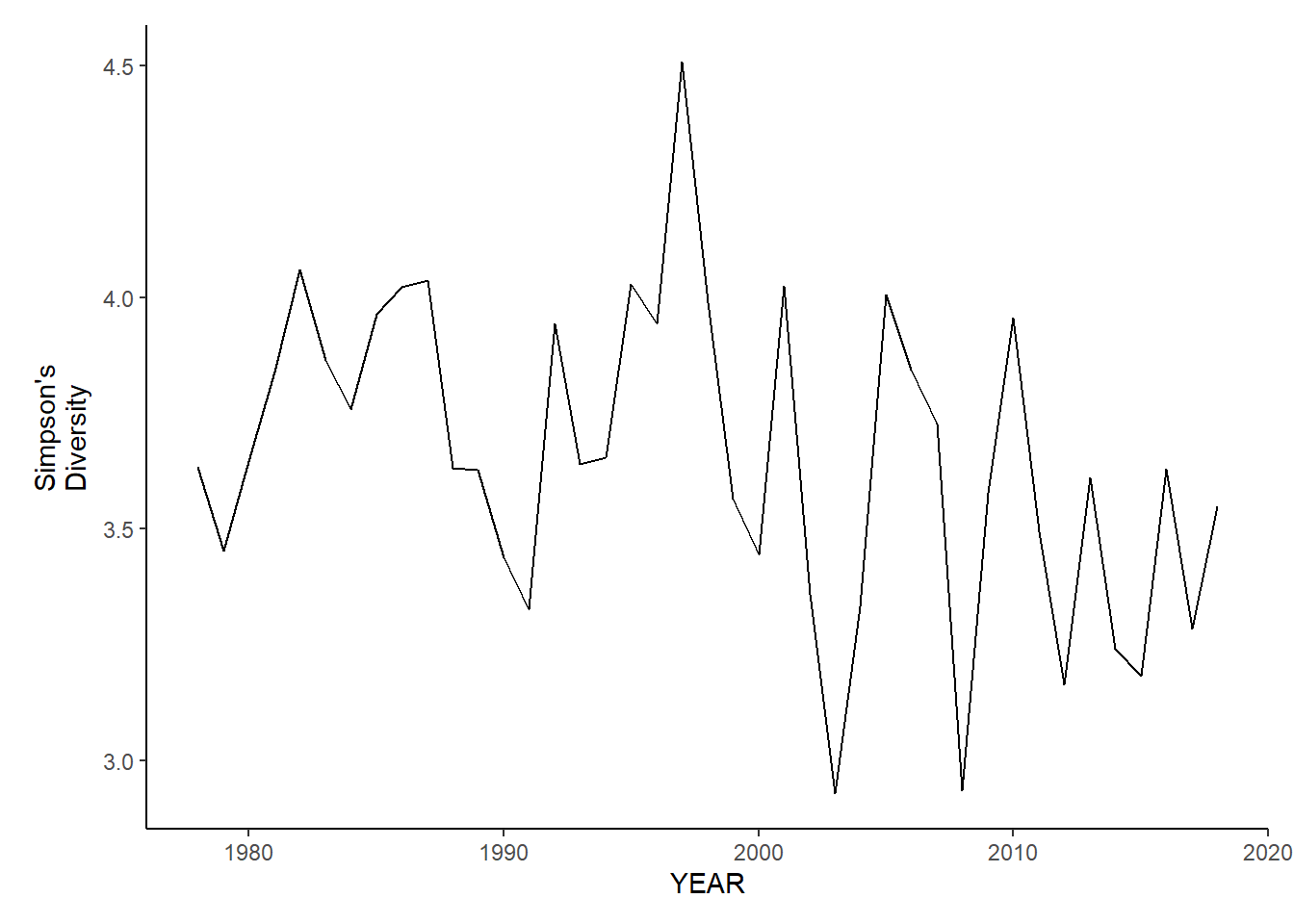

ma_fl_simpson.d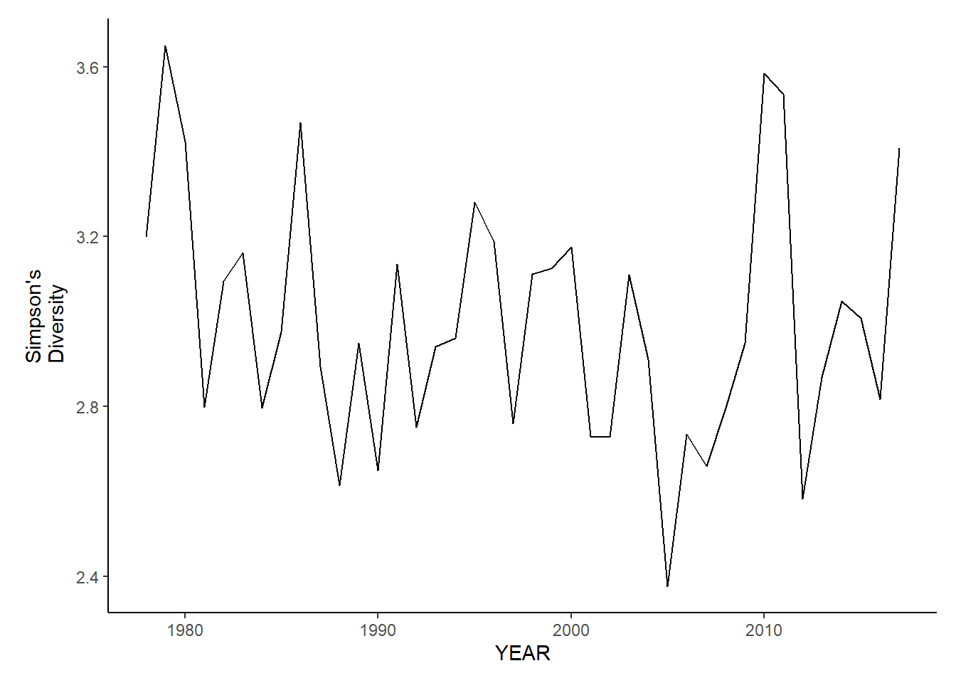

Simpson’s evenness

ma_sp_simpson.e<-ggplot()+geom_line(data=ma_spring_inds, aes(YEAR, avg_E_index))+theme_classic()+ylab(expression(paste("Simpson's\nEvenness")))+theme(plot.margin = margin(10, 10, 10, 25))
                                   
ma_fl_simpson.e<-ggplot()+geom_line(data=ma_fall_inds, aes(YEAR, avg_E_index))+theme_classic()+ylab(expression(paste("Simpson's\nEvenness")))+theme(plot.margin = margin(10, 10, 10, 25)) 

ma_sp_simpson.e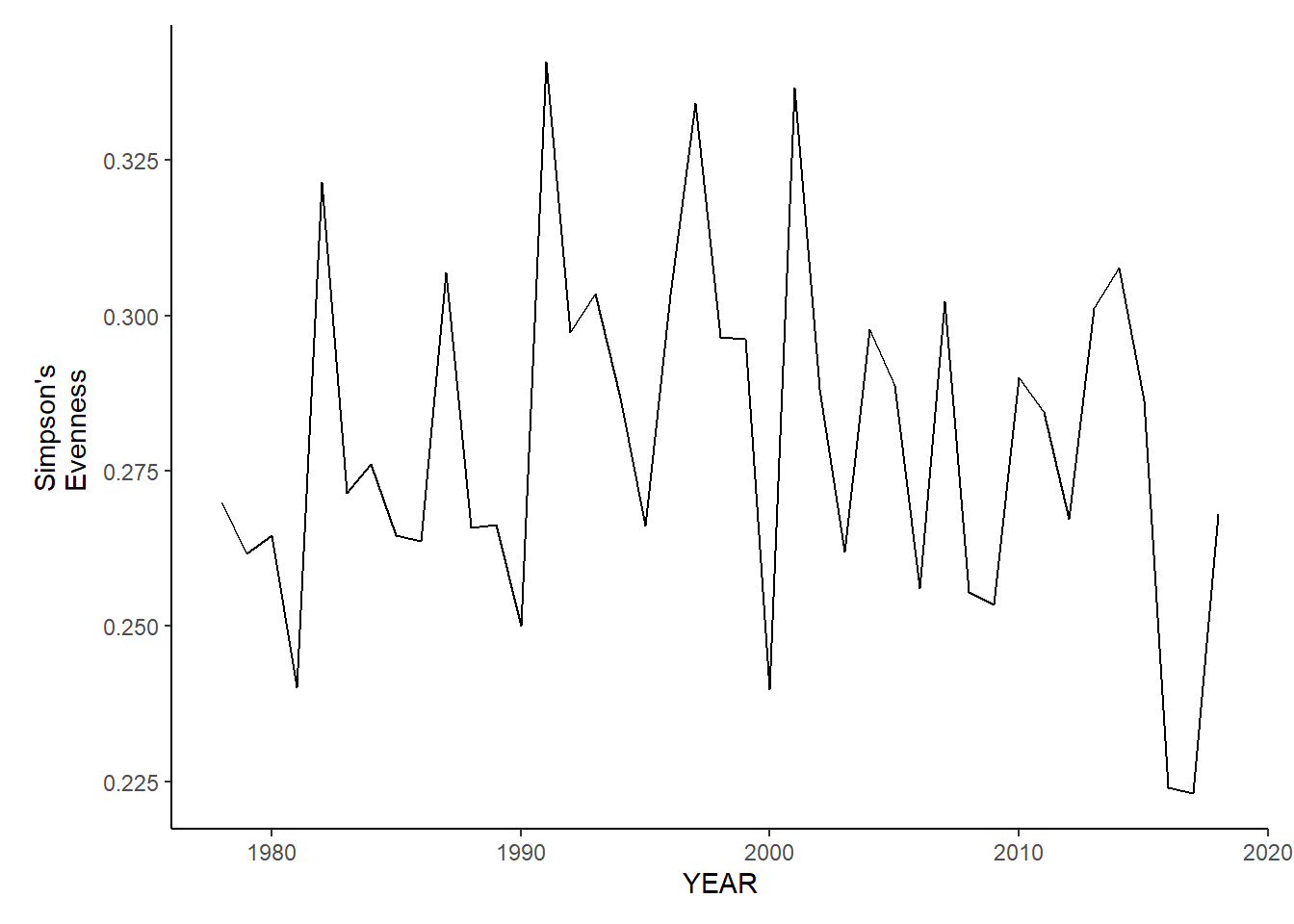

ma_fl_simpson.e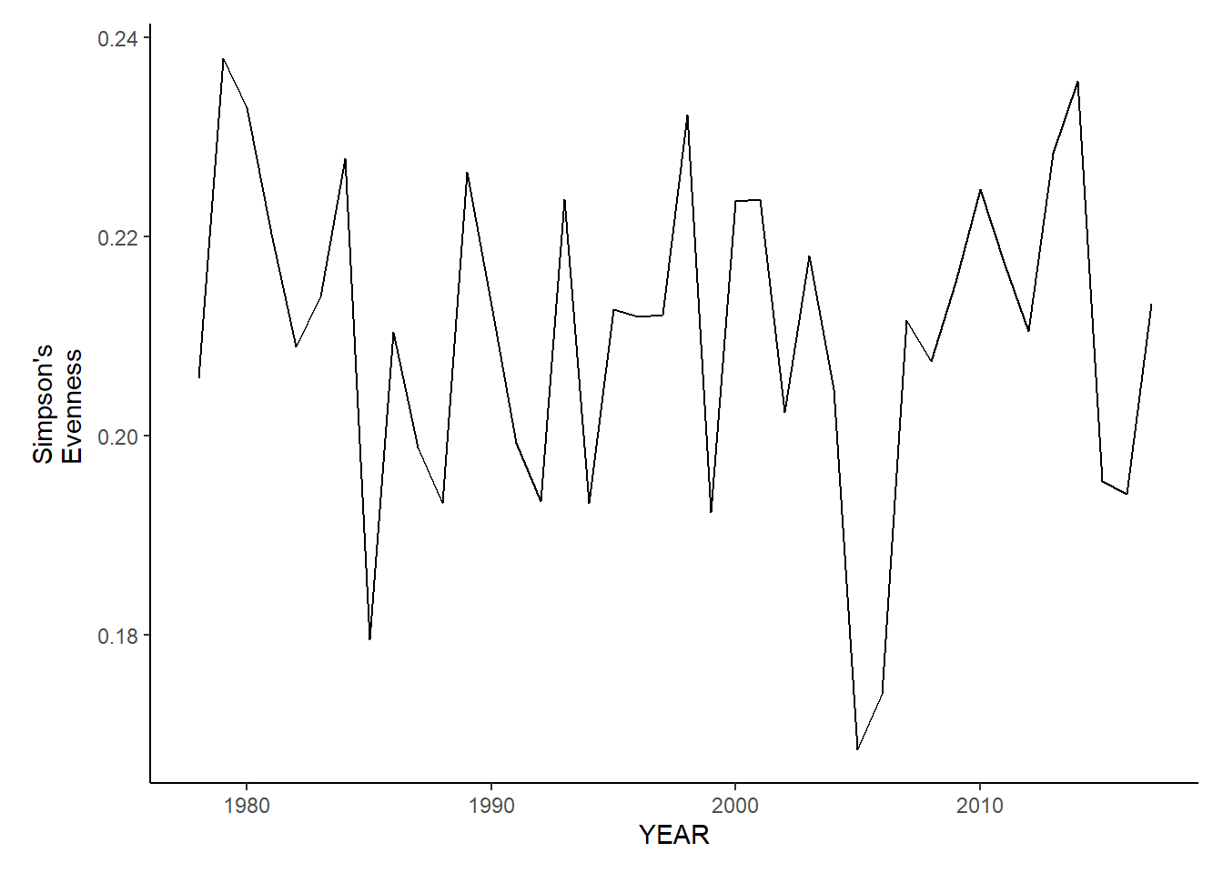

Taxonomic diversity

ma_sp_tax.diversity<-ggplot()+geom_line(data=ma_spring_inds, aes(YEAR, avg_delta))+theme_classic()+ylab(expression(paste("Taxonomic\nDiversity")))+theme(plot.margin = margin(10, 10, 10, 25))
                                   
ma_fl_tax.diversity<-ggplot()+geom_line(data=ma_fall_inds, aes(YEAR, avg_delta))+theme_classic()+ylab(expression(paste("Taxonomic\nDiversity")))+theme(plot.margin = margin(10, 10, 10, 25)) 

ma_sp_tax.diversity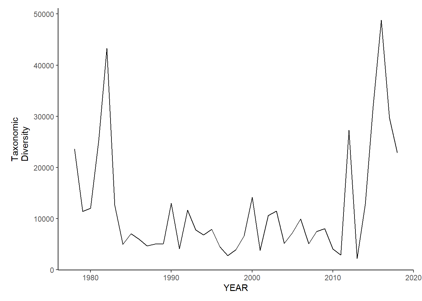

ma_fl_tax.diversity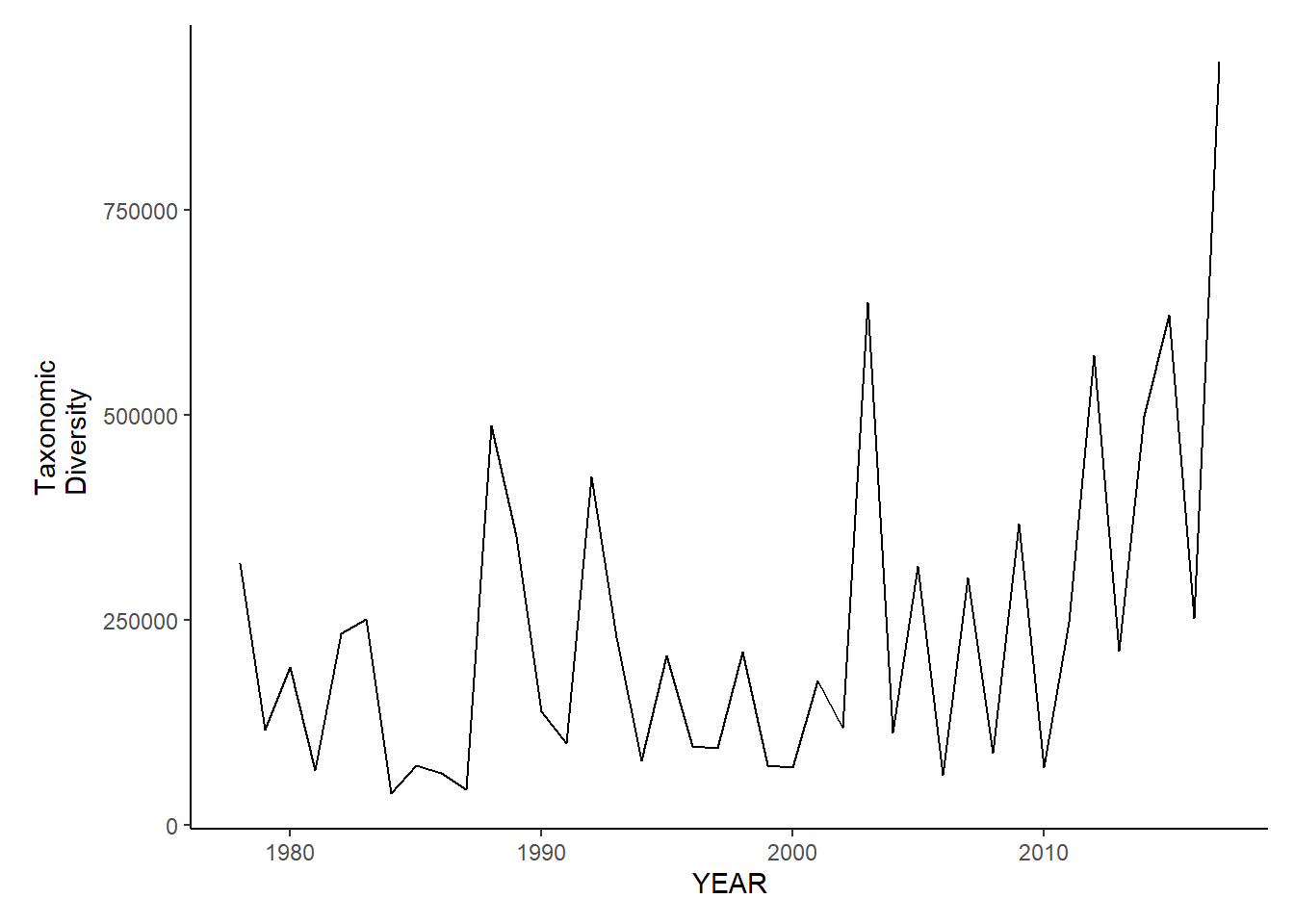

Taxonomic distinctness

ma_sp_tax.distinct<-ggplot()+geom_line(data=ma_spring_inds, aes(YEAR, avg_delta_star))+theme_classic()+ylab(expression(paste("Taxonomic\nDistinctness")))+theme(plot.margin = margin(10, 10, 10, 25))
                                   
ma_fl_tax.distinct<-ggplot()+geom_line(data=ma_fall_inds, aes(YEAR, avg_delta_star))+theme_classic()+ylab(expression(paste("Taxonomic\nDistinctness")))+theme(plot.margin = margin(10, 10, 10, 25)) 

ma_sp_tax.distinct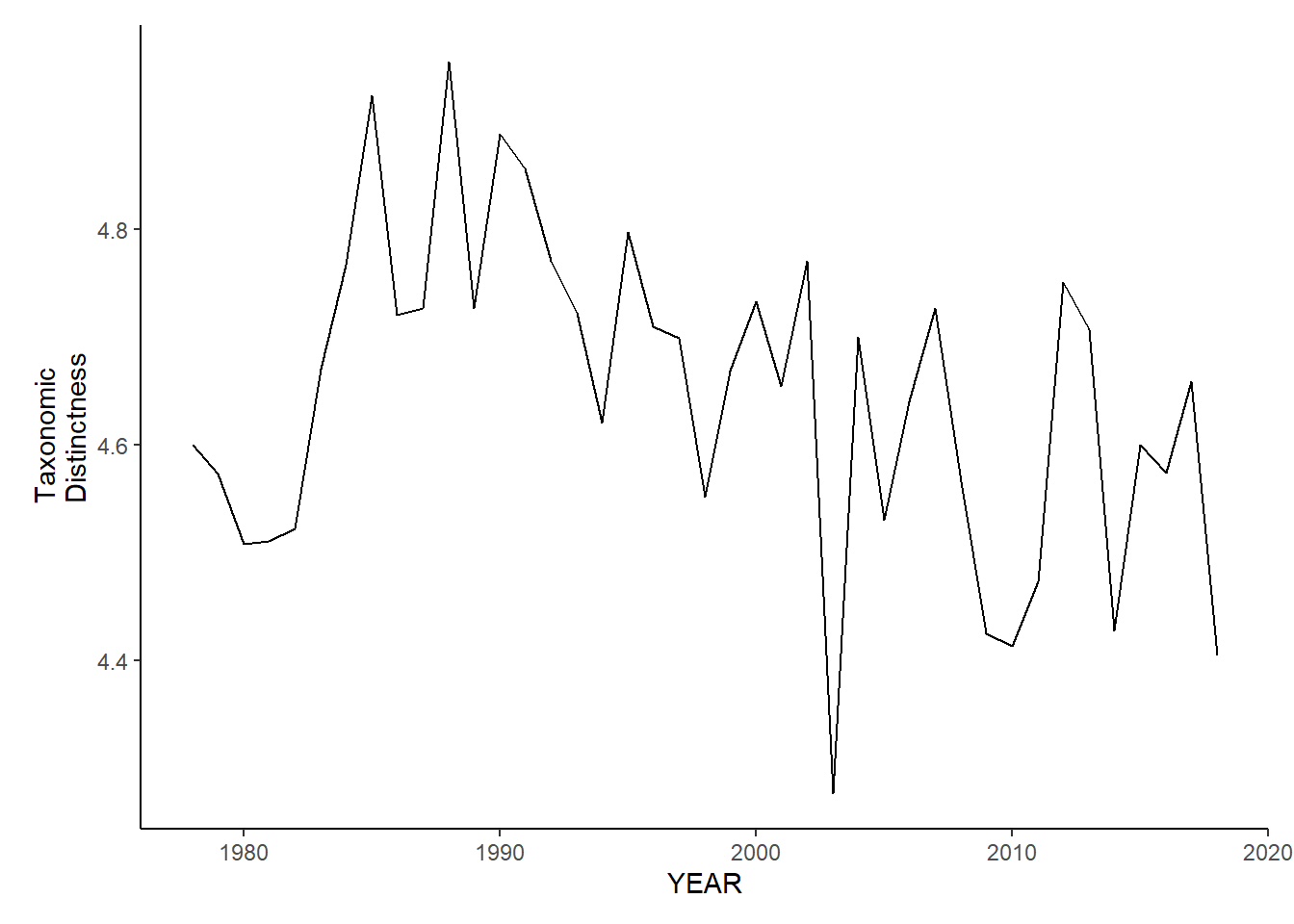

ma_fl_tax.distinct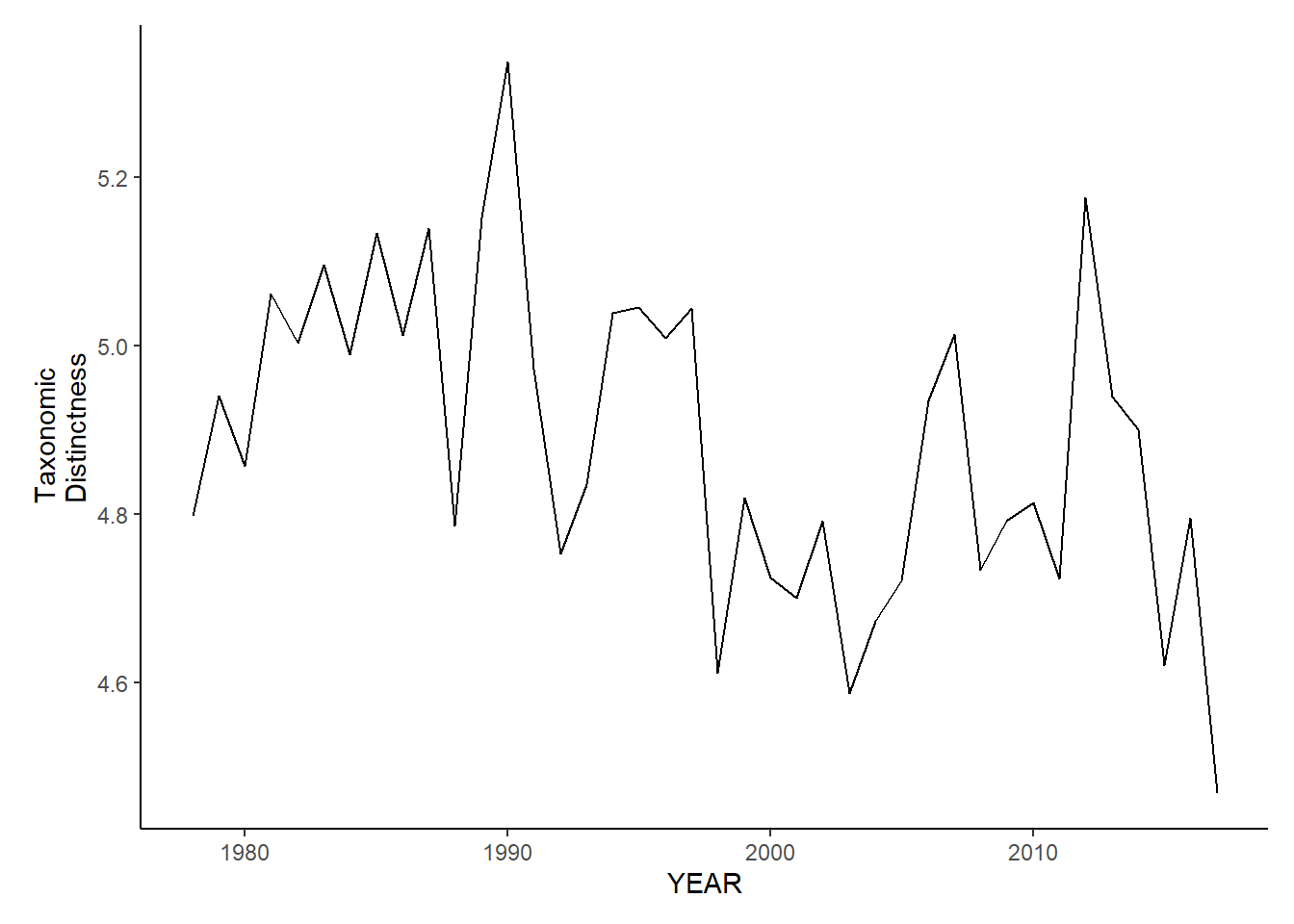

Average taxonomic distinctness

ma_sp_avg.tax.distinct<-ggplot()+geom_line(data=ma_spring_inds, aes(YEAR, avg_delta_plus))+theme_classic()+ylab(expression(paste("Average\nTaxonomic\nDistinctness")))+theme(plot.margin = margin(10, 10, 10, 25))
                                   
ma_fl_avg.tax.distinct<-ggplot()+geom_line(data=ma_fall_inds, aes(YEAR, avg_delta_plus))+theme_classic()+ylab(expression(paste("Average\nTaxonomic\nDistinctness")))+theme(plot.margin = margin(10, 10, 10, 25)) 

ma_sp_avg.tax.distinct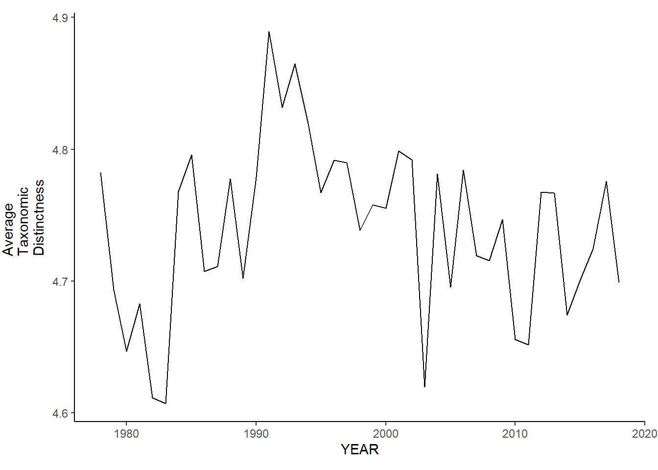

ma_fl_avg.tax.distinct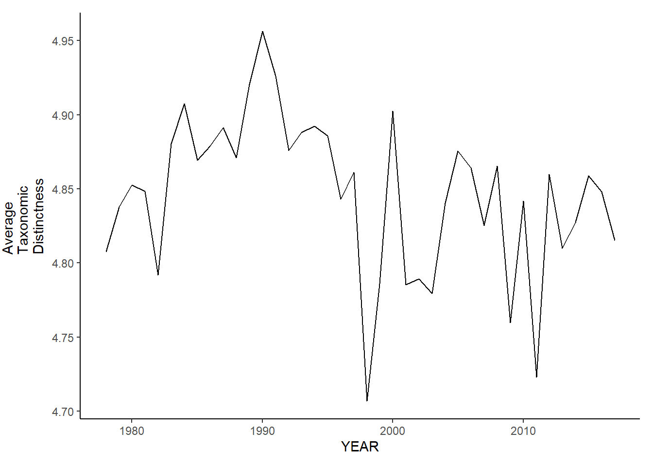

Variation in taxonomic distinctness

ma_sp_var.tax.distinct<-ggplot()+geom_line(data=ma_spring_inds, aes(YEAR, avg_delta_var))+theme_classic()+ylab(expression(paste("Variation\nTaxonomic\nDistinctness")))+theme(plot.margin = margin(10, 10, 10, 25))
                                   
ma_fl_var.tax.distinct<-ggplot()+geom_line(data=ma_fall_inds, aes(YEAR, avg_delta_var))+theme_classic()+ylab(expression(paste("Variation\nTaxonomic\nDistinctness")))+theme(plot.margin = margin(10, 10, 10, 25)) 

ma_sp_var.tax.distinct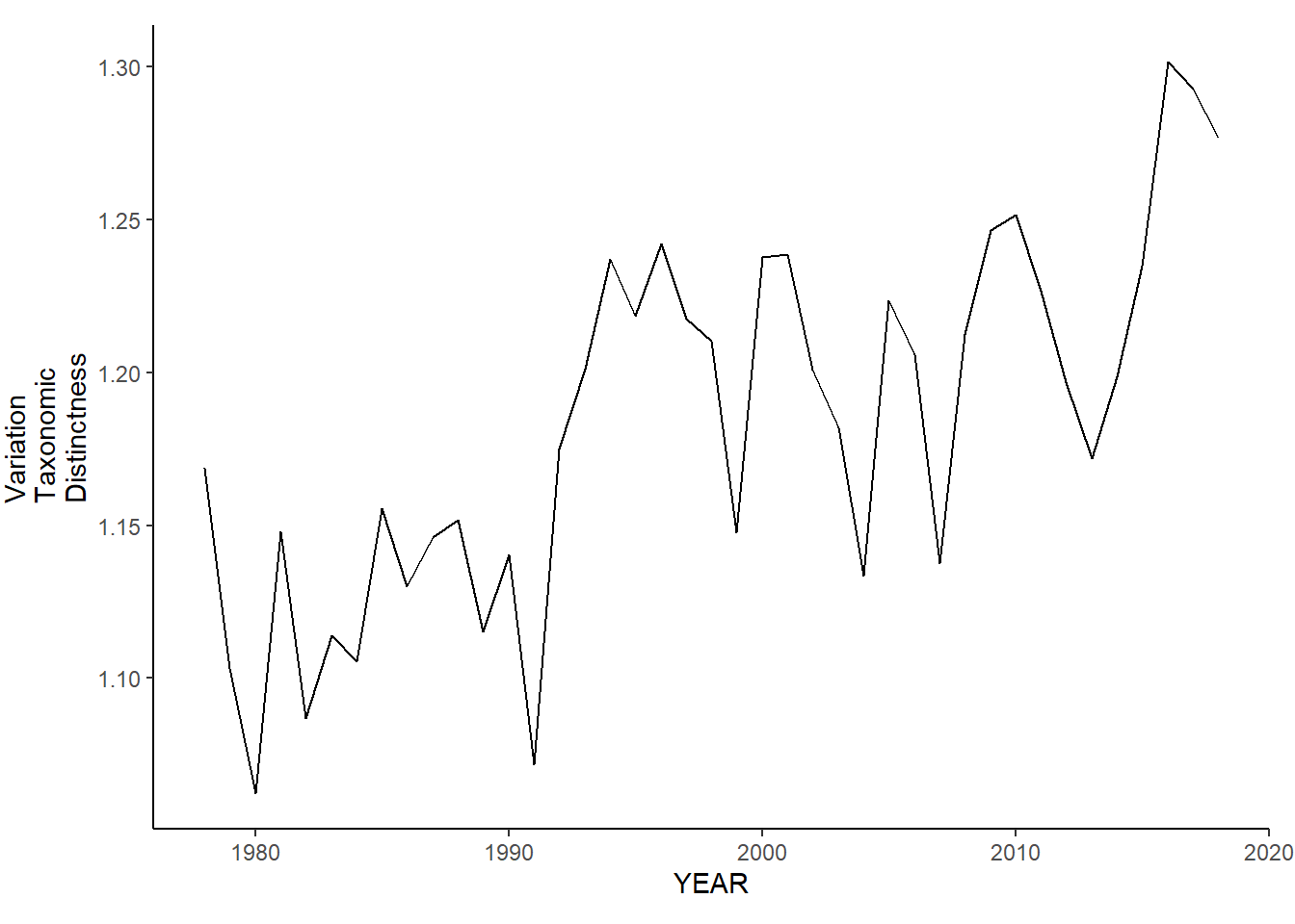

ma_fl_var.tax.distinct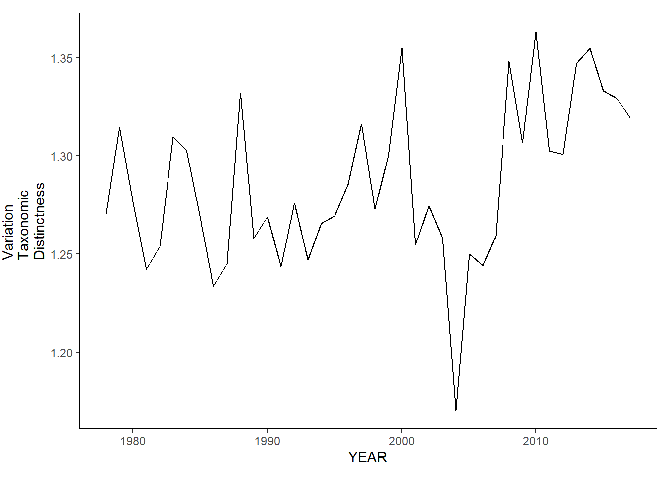

NEFSC Bottom Trawl survey biodiversity metrics

setwd("C:/Users/jjesse/Box/Kerr Lab/Fisheries Science Lab/ME NH Trawl- Seagrant/Seagrant-AEW/NEFSC")
nefsc_spring_inds<-read.csv("NEFSC_all_metrics_SP.csv")%>%
  rename(YEAR=EST_YEAR)%>%
  group_by(YEAR)%>%
  summarise(avg_N_species=mean(N_species, na.rm=TRUE), avg_H_index=mean(H_index, na.rm=TRUE), avg_D_index=mean(D_index, na.rm=TRUE), avg_E_index=mean(E_index, na.rm=TRUE), avg_delta=mean(delta, na.rm=TRUE), avg_delta_star=mean(delta_star, na.rm=TRUE), avg_delta_plus=mean(delta_plus, na.rm=TRUE), avg_delta_var=mean(delta_var, na.rm=TRUE))

nefsc_fall_inds<-read.csv("NEFSC_all_metrics_FL.csv")%>%
  rename(YEAR=EST_YEAR)%>%
  group_by(YEAR)%>%
  summarise(avg_N_species=mean(N_species, na.rm=TRUE), avg_H_index=mean(H_index, na.rm=TRUE), avg_D_index=mean(D_index, na.rm=TRUE), avg_E_index=mean(E_index, na.rm=TRUE), avg_delta=mean(delta, na.rm=TRUE), avg_delta_star=mean(delta_star, na.rm=TRUE), avg_delta_plus=mean(delta_plus, na.rm=TRUE), avg_delta_var=mean(delta_var, na.rm=TRUE))

Species richness

nefsc_sp_richness<-ggplot()+geom_line(data=nefsc_spring_inds, aes(YEAR, avg_N_species))+theme_classic()+ylab(expression(paste("Species\nRichness")))+theme(plot.margin = margin(10, 10, 10, 25))
                                   
nefsc_fl_richness<-ggplot()+geom_line(data=nefsc_fall_inds, aes(YEAR, avg_N_species))+theme_classic()+ylab(expression(paste("Species\nRichness")))+theme(plot.margin = margin(10, 10, 10, 25)) 

nefsc_sp_richness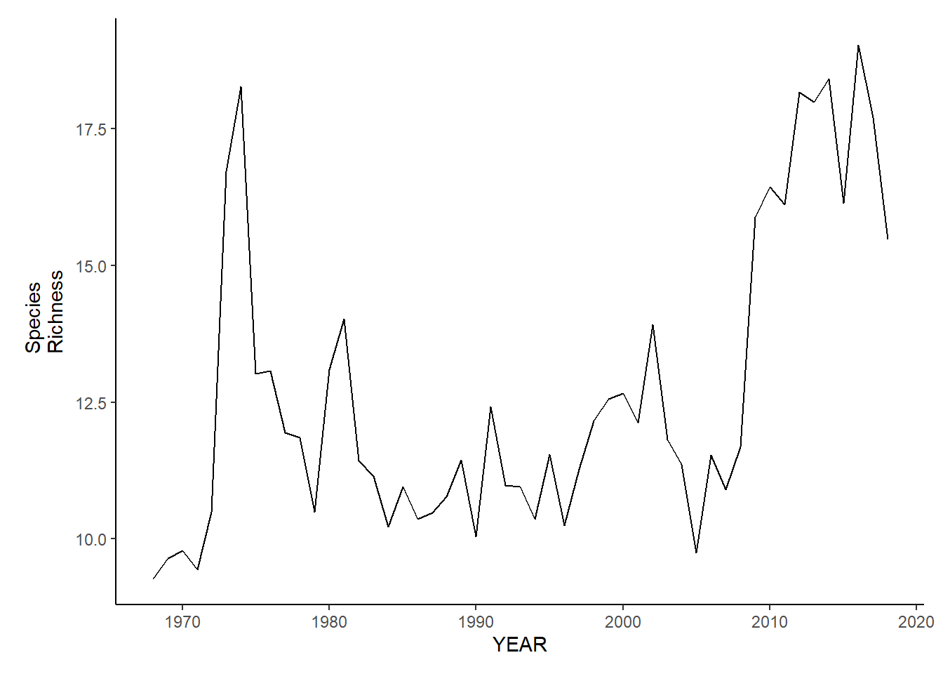

nefsc_fl_richness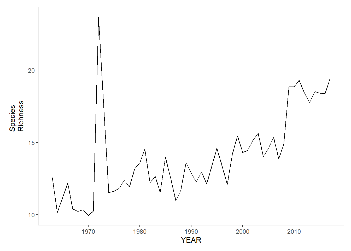

Shannon-Weiner diversity

nefsc_sp_shannon<-ggplot()+geom_line(data=nefsc_spring_inds, aes(YEAR, avg_H_index))+theme_classic()+ylab(expression(paste("Simpson's\nEvenness")))+theme(plot.margin = margin(10, 10, 10, 25))
                                   
nefsc_fl_shannon<-ggplot()+geom_line(data=nefsc_fall_inds, aes(YEAR, avg_H_index))+theme_classic()+ylab(expression(paste("Simpson's\nEvenness")))+theme(plot.margin = margin(10, 10, 10, 25)) 

nefsc_sp_shannon

nefsc_fl_shannon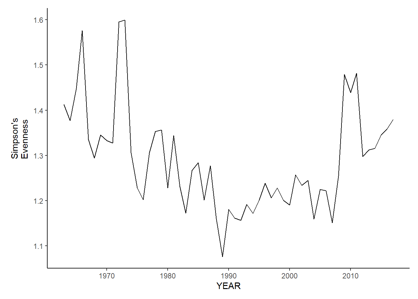

Simpson’s diversity

nefsc_sp_simpson.d<-ggplot()+geom_line(data=nefsc_spring_inds, aes(YEAR, avg_D_index))+theme_classic()+ylab(expression(paste("Simpson's\nDiversity")))+theme(plot.margin = margin(10, 10, 10, 25))
                                   
nefsc_fl_simpson.d<-ggplot()+geom_line(data=nefsc_fall_inds, aes(YEAR, avg_D_index))+theme_classic()+ylab(expression(paste("Simpson's\nDiversity")))+theme(plot.margin = margin(10, 10, 10, 25)) 

nefsc_sp_simpson.d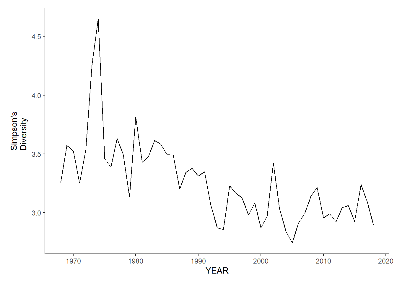

nefsc_fl_simpson.d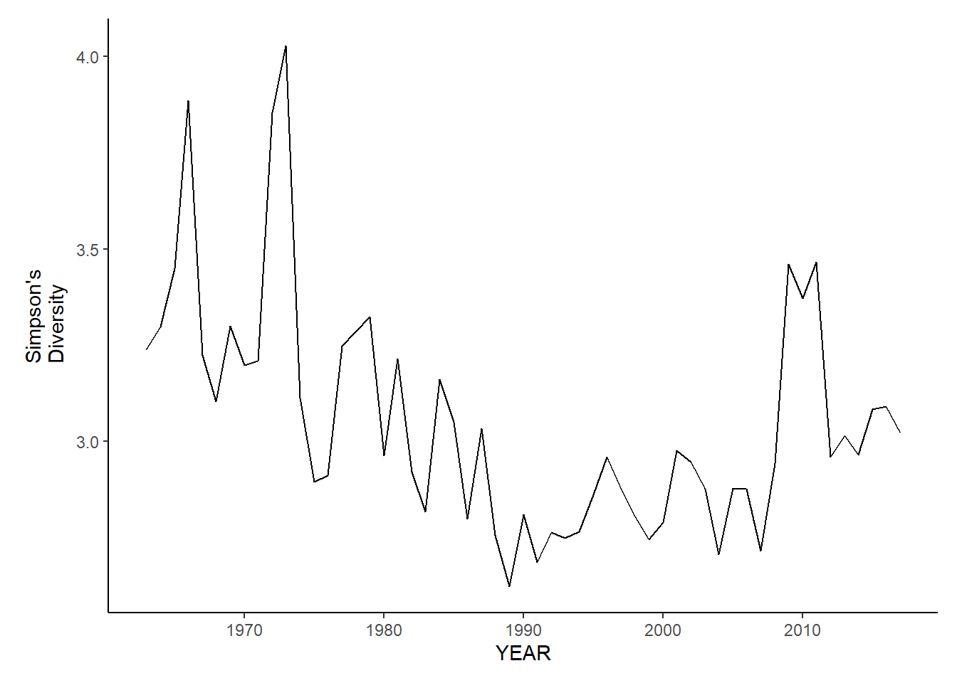

Simpson’s evenness

nefsc_sp_simpson.e<-ggplot()+geom_line(data=nefsc_spring_inds, aes(YEAR, avg_E_index))+theme_classic()+ylab(expression(paste("Simpson's\nEvenness")))+theme(plot.margin = margin(10, 10, 10, 25))
                                   
nefsc_fl_simpson.e<-ggplot()+geom_line(data=nefsc_fall_inds, aes(YEAR, avg_E_index))+theme_classic()+ylab(expression(paste("Simpson's\nEvenness")))+theme(plot.margin = margin(10, 10, 10, 25)) 

nefsc_sp_simpson.e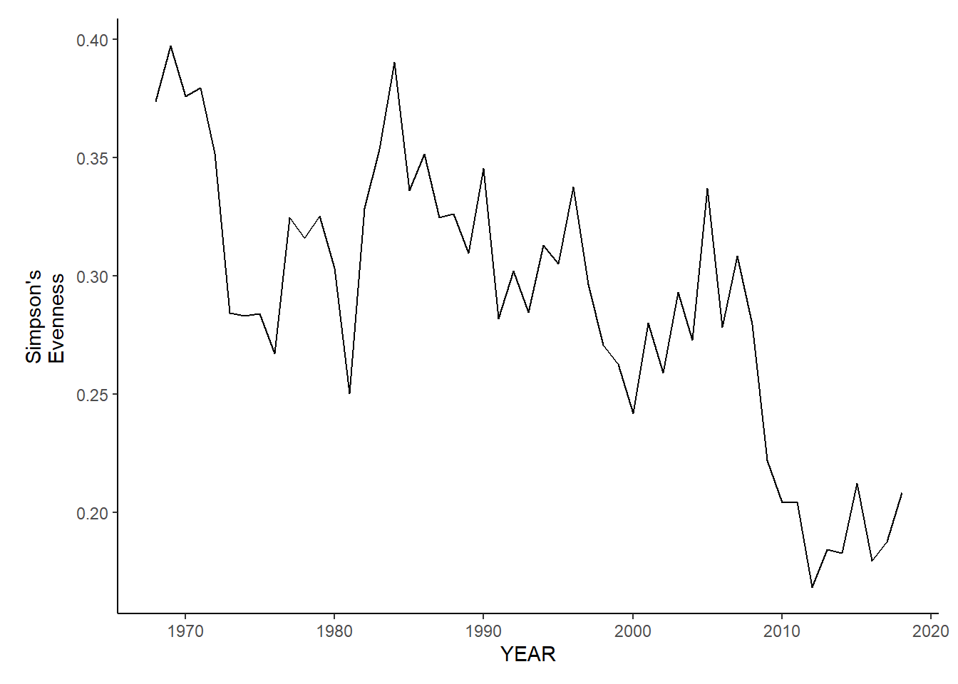

nefsc_fl_simpson.e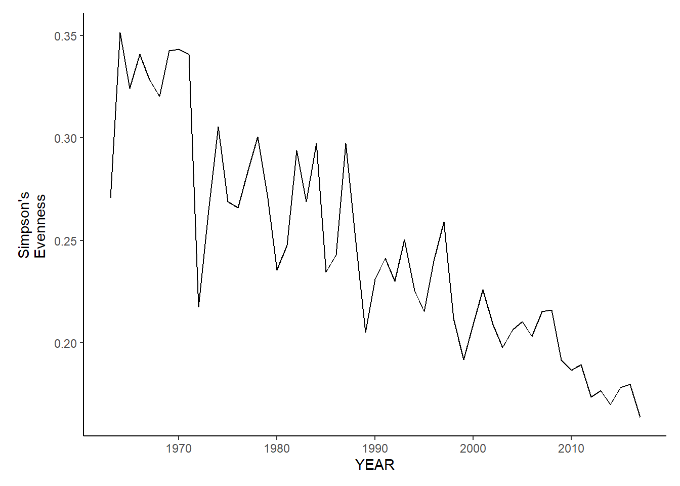

Taxonomic diversity

nefsc_sp_tax.diversity<-ggplot()+geom_line(data=nefsc_spring_inds, aes(YEAR, avg_delta))+theme_classic()+ylab(expression(paste("Taxonomic\nDiversity")))+theme(plot.margin = margin(10, 10, 10, 25))
                                   
nefsc_fl_tax.diversity<-ggplot()+geom_line(data=nefsc_fall_inds, aes(YEAR, avg_delta))+theme_classic()+ylab(expression(paste("Taxonomic\nDiversity")))+theme(plot.margin = margin(10, 10, 10, 25)) 

nefsc_sp_tax.diversity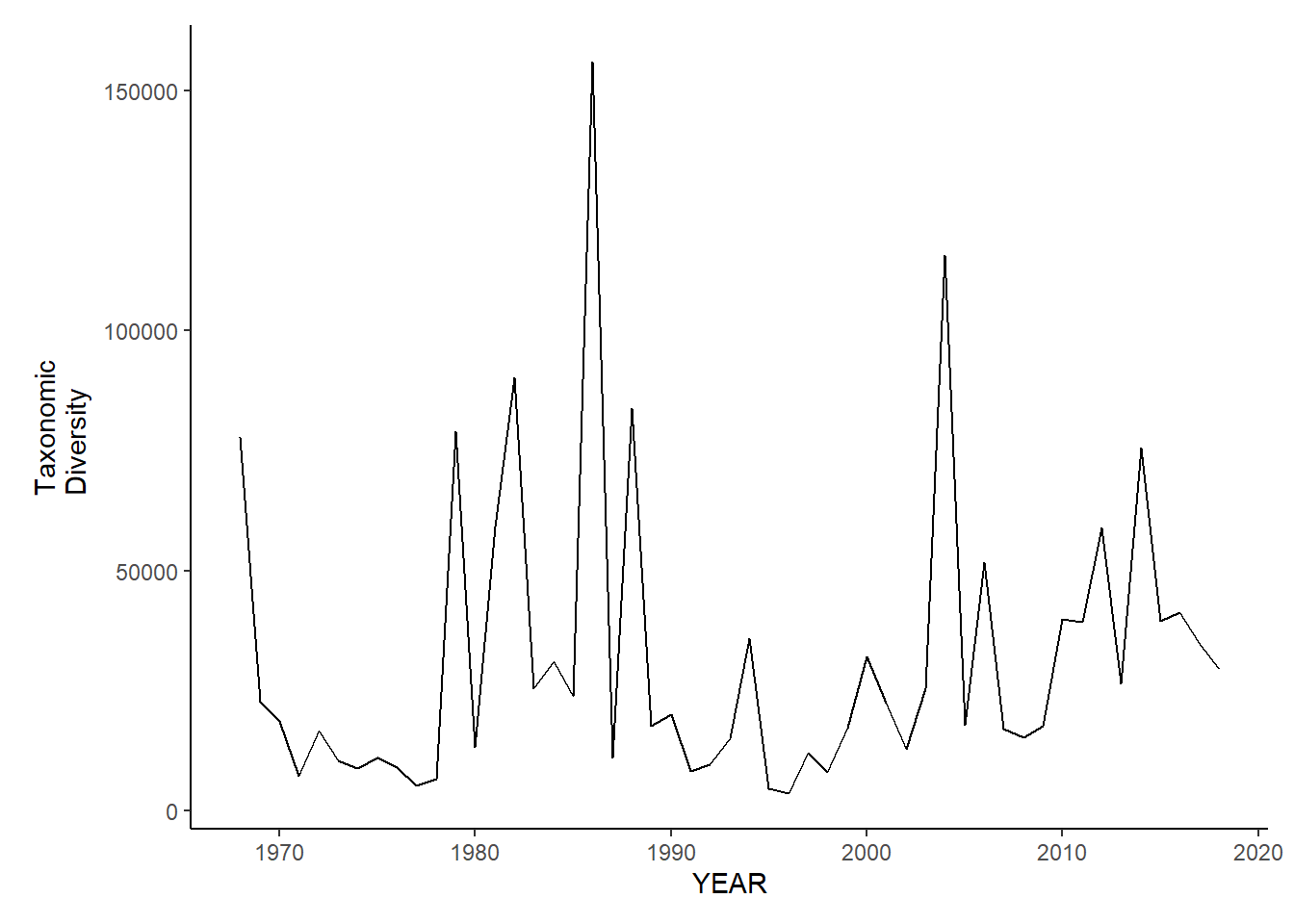

nefsc_fl_tax.diversity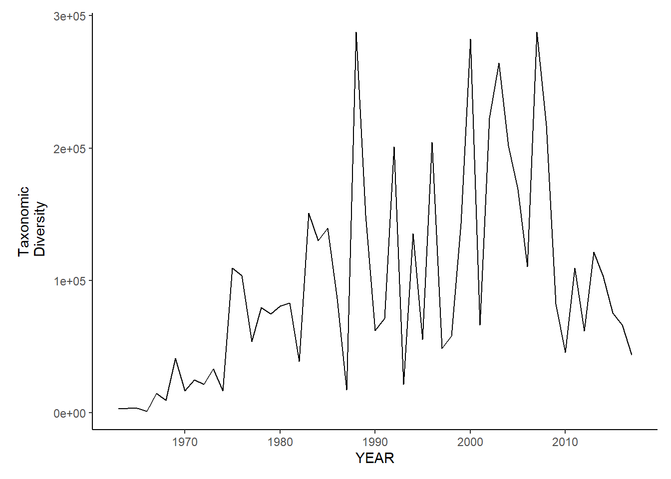

Taxonomic distinctness

nefsc_sp_tax.distinct<-ggplot()+geom_line(data=nefsc_spring_inds, aes(YEAR, avg_delta_star))+theme_classic()+ylab(expression(paste("Taxonomic\nDistinctness")))+theme(plot.margin = margin(10, 10, 10, 25))
                                   
nefsc_fl_tax.distinct<-ggplot()+geom_line(data=nefsc_fall_inds, aes(YEAR, avg_delta_star))+theme_classic()+ylab(expression(paste("Taxonomic\nDistinctness")))+theme(plot.margin = margin(10, 10, 10, 25)) 

nefsc_sp_tax.distinct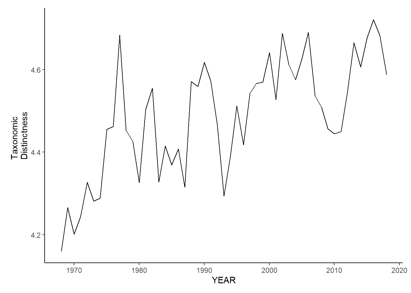

nefsc_fl_tax.distinct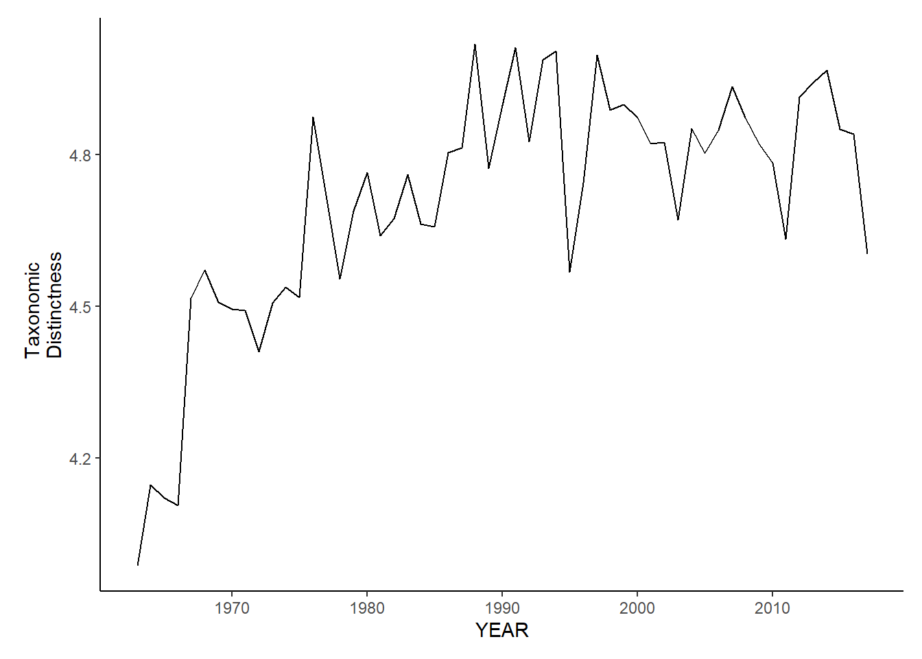

Average taxonomic distinctness

nefsc_sp_avg.tax.distinct<-ggplot()+geom_line(data=nefsc_spring_inds, aes(YEAR, avg_delta_plus))+theme_classic()+ylab(expression(paste("Average\nTaxonomic\nDistinctness")))+theme(plot.margin = margin(10, 10, 10, 25))
                                   
nefsc_fl_avg.tax.distinct<-ggplot()+geom_line(data=nefsc_fall_inds, aes(YEAR, avg_delta_plus))+theme_classic()+ylab(expression(paste("Average\nTaxonomic\nDistinctness")))+theme(plot.margin = margin(10, 10, 10, 25)) 

nefsc_sp_avg.tax.distinct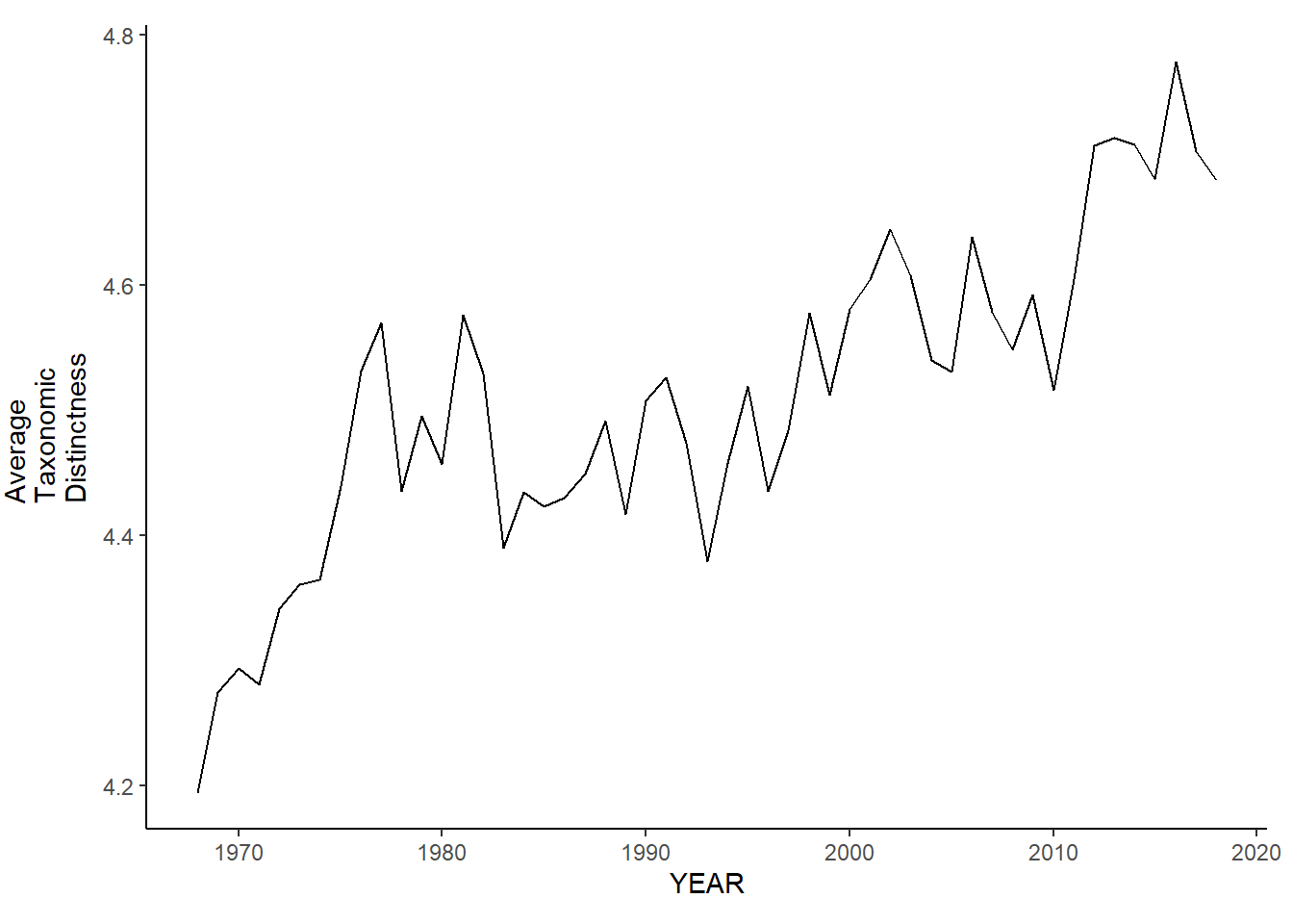

nefsc_fl_avg.tax.distinct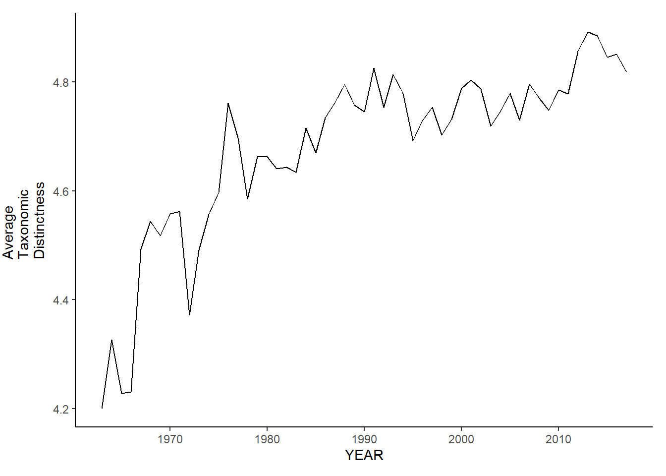

Variation in taxonomic distinctness

nefsc_sp_var.tax.distinct<-ggplot()+geom_line(data=nefsc_spring_inds, aes(YEAR, avg_delta_var))+theme_classic()+ylab(expression(paste("Variation\nTaxonomic\nDistinctness")))+theme(plot.margin = margin(10, 10, 10, 25))
                                   
nefsc_fl_var.tax.distinct<-ggplot()+geom_line(data=nefsc_fall_inds, aes(YEAR, avg_delta_var))+theme_classic()+ylab(expression(paste("Variation\nTaxonomic\nDistinctness")))+theme(plot.margin = margin(10, 10, 10, 25)) 

nefsc_sp_var.tax.distinct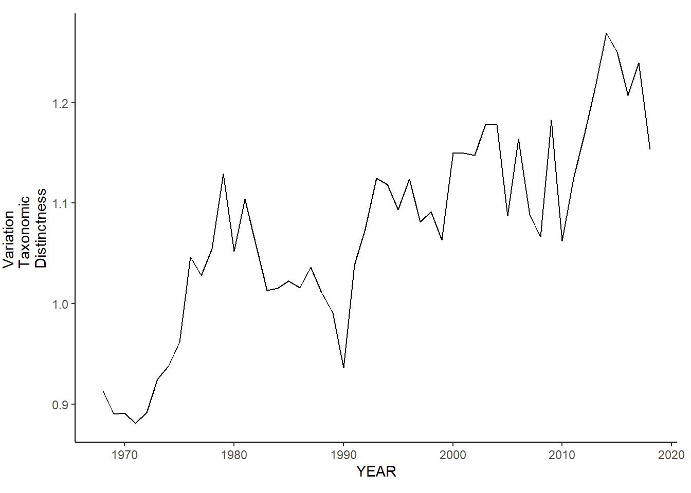

nefsc_fl_var.tax.distinct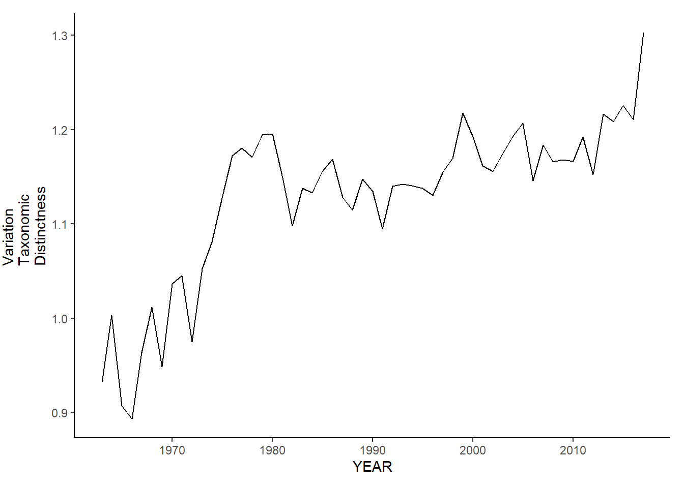

GOM/GB NEFSC Trawl Survey biodiversity metrics

setwd("C:/Users/jjesse/Box/Kerr Lab/Fisheries Science Lab/ME NH Trawl- Seagrant/Seagrant-AEW/NEFSC")
gom_spring_inds<-read.csv("GOM_spring.csv")%>%
  rename(YEAR=EST_YEAR)%>%
  group_by(YEAR)%>%
  summarise(avg_N_species=mean(N_species, na.rm=TRUE), avg_H_index=mean(H_index, na.rm=TRUE), avg_D_index=mean(D_index, na.rm=TRUE), avg_E_index=mean(E_index, na.rm=TRUE), avg_delta=mean(delta, na.rm=TRUE), avg_delta_star=mean(delta_star, na.rm=TRUE), avg_delta_plus=mean(delta_plus, na.rm=TRUE), avg_delta_var=mean(delta_var, na.rm=TRUE))

gom_fall_inds<-read.csv("GOM_fall.csv")%>%
  rename(YEAR=EST_YEAR)%>%
  group_by(YEAR)%>%
  summarise(avg_N_species=mean(N_species, na.rm=TRUE), avg_H_index=mean(H_index, na.rm=TRUE), avg_D_index=mean(D_index, na.rm=TRUE), avg_E_index=mean(E_index, na.rm=TRUE), avg_delta=mean(delta, na.rm=TRUE), avg_delta_star=mean(delta_star, na.rm=TRUE), avg_delta_plus=mean(delta_plus, na.rm=TRUE), avg_delta_var=mean(delta_var, na.rm=TRUE))

Species richness

gom_sp_richness<-ggplot()+geom_line(data=gom_spring_inds, aes(YEAR, avg_N_species))+theme_classic()+ylab(expression(paste("Species\nRichness")))+theme(plot.margin = margin(10, 10, 10, 25))
                                   
gom_fl_richness<-ggplot()+geom_line(data=gom_fall_inds, aes(YEAR, avg_N_species))+theme_classic()+ylab(expression(paste("Species\nRichness")))+theme(plot.margin = margin(10, 10, 10, 25)) 

gom_sp_richness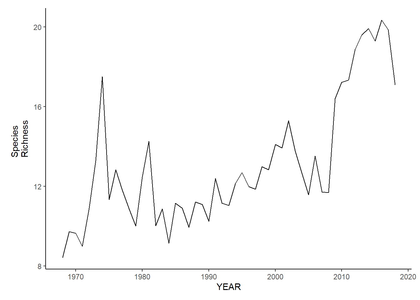

gom_fl_richness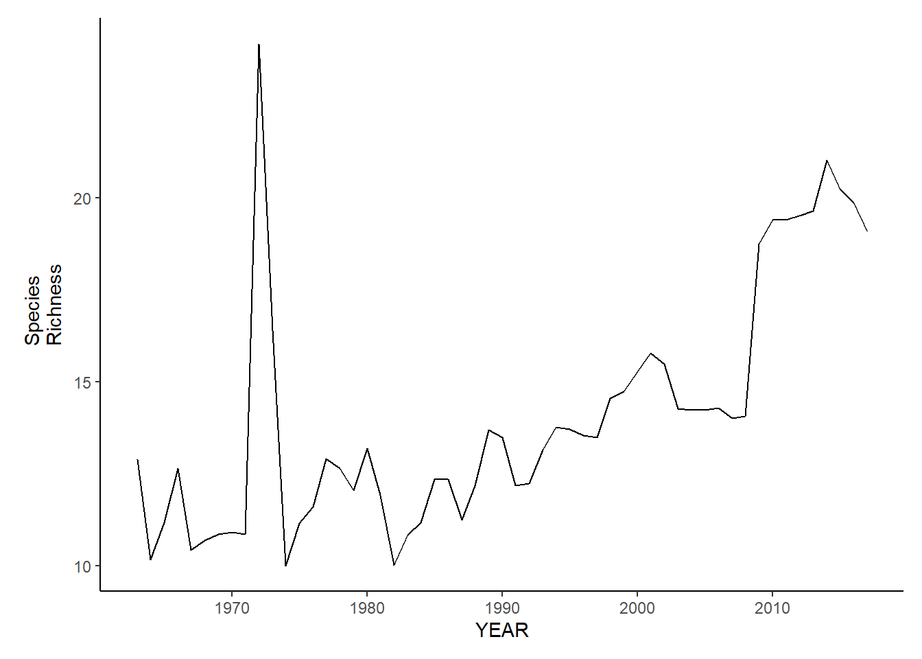

Shannon-Weiner diversity

gom_sp_shannon<-ggplot()+geom_line(data=gom_spring_inds, aes(YEAR, avg_H_index))+theme_classic()+ylab(expression(paste("Simpson's\nEvenness")))+theme(plot.margin = margin(10, 10, 10, 25))
                                   
gom_fl_shannon<-ggplot()+geom_line(data=gom_fall_inds, aes(YEAR, avg_H_index))+theme_classic()+ylab(expression(paste("Simpson's\nEvenness")))+theme(plot.margin = margin(10, 10, 10, 25)) 

gom_sp_shannon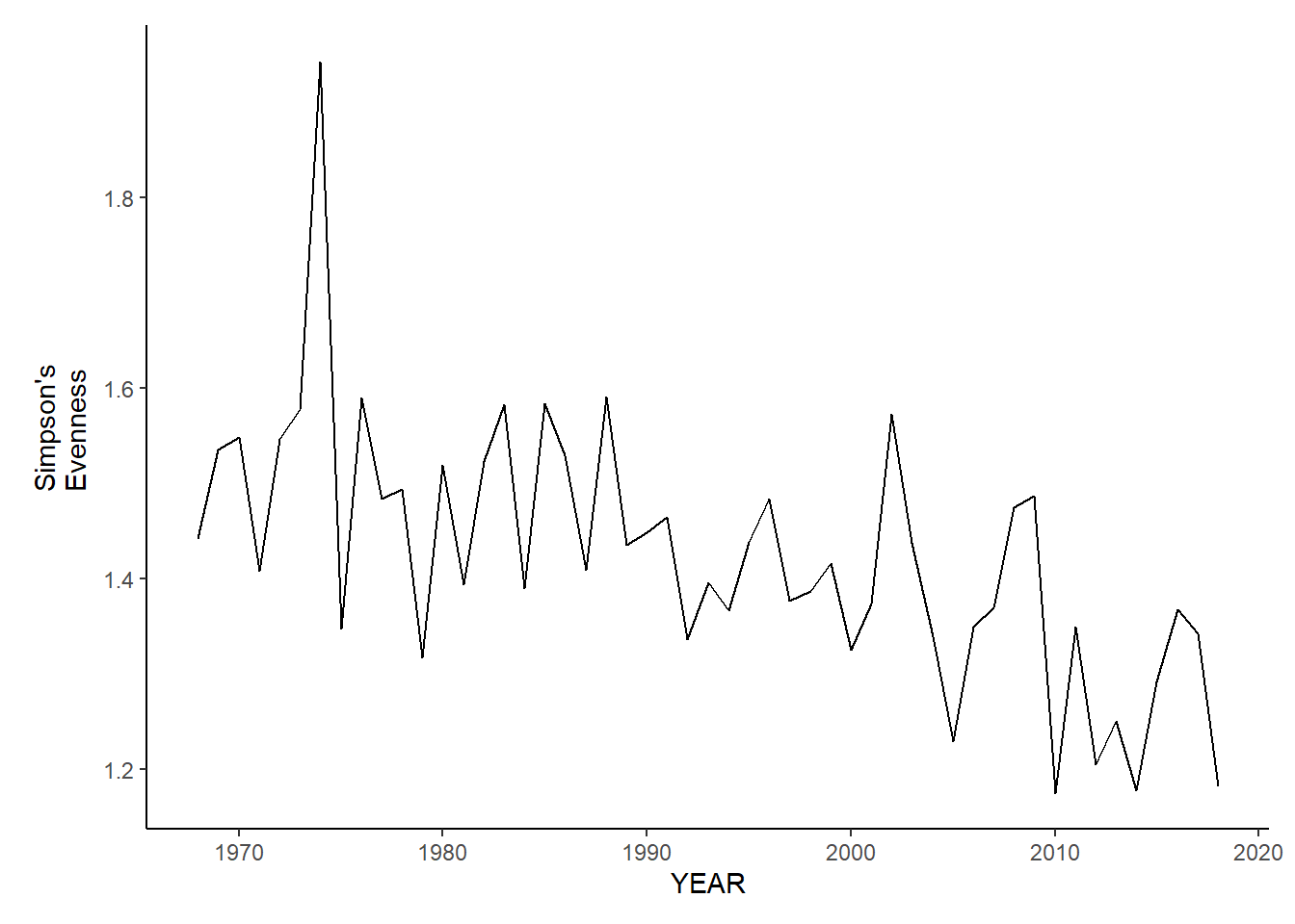

gom_fl_shannon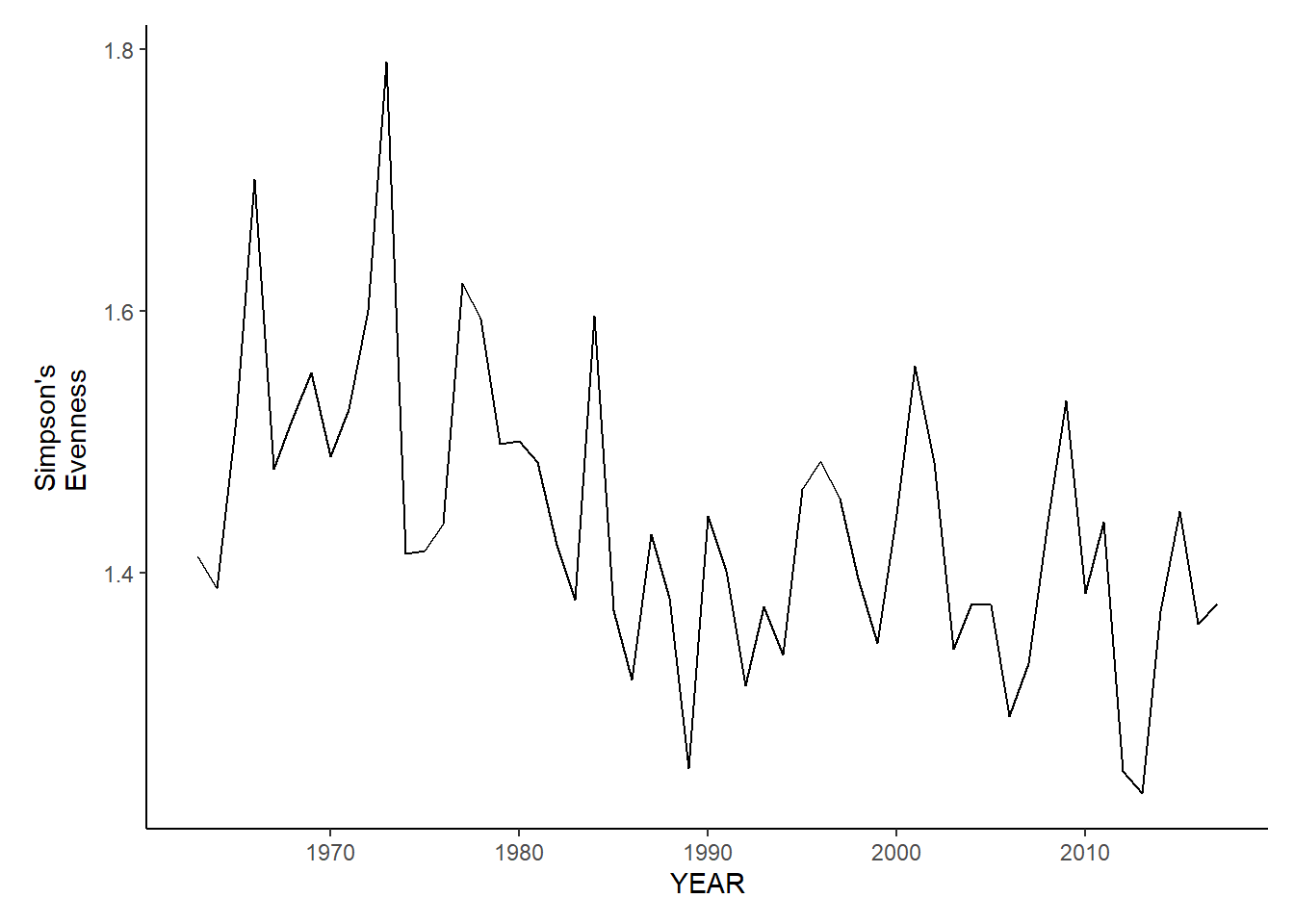

Simpson’s diversity

gom_sp_simpson.d<-ggplot()+geom_line(data=gom_spring_inds, aes(YEAR, avg_D_index))+theme_classic()+ylab(expression(paste("Simpson's\nDiversity")))+theme(plot.margin = margin(10, 10, 10, 25))
                                   
gom_fl_simpson.d<-ggplot()+geom_line(data=gom_fall_inds, aes(YEAR, avg_D_index))+theme_classic()+ylab(expression(paste("Simpson's\nDiversity")))+theme(plot.margin = margin(10, 10, 10, 25)) 

gom_sp_simpson.d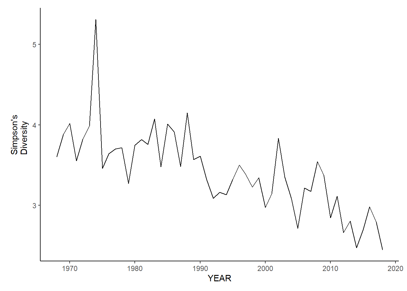

gom_fl_simpson.d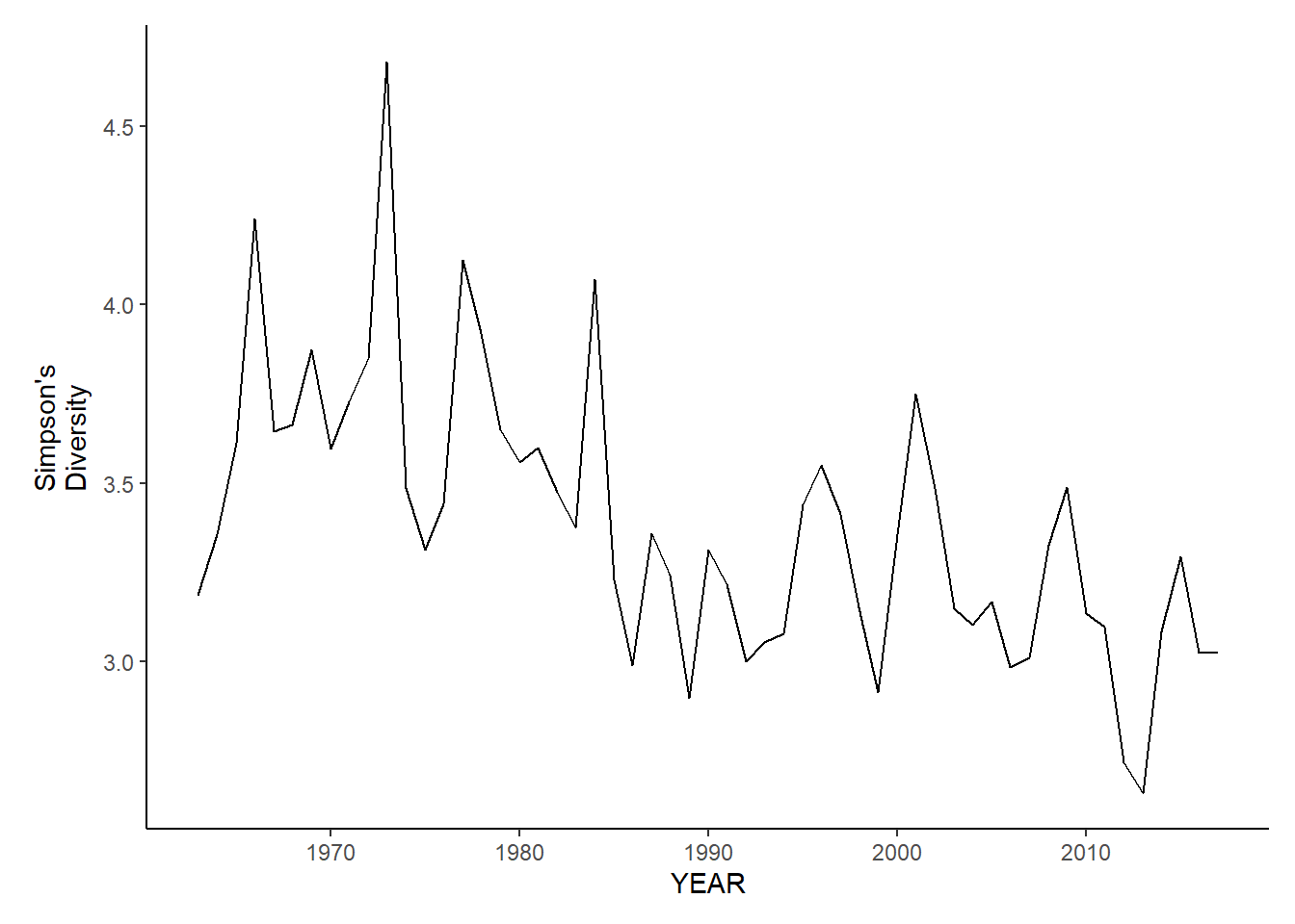

Simpson’s evenness

gom_sp_simpson.e<-ggplot()+geom_line(data=gom_spring_inds, aes(YEAR, avg_E_index))+theme_classic()+ylab(expression(paste("Simpson's\nEvenness")))+theme(plot.margin = margin(10, 10, 10, 25))
                                   
gom_fl_simpson.e<-ggplot()+geom_line(data=gom_fall_inds, aes(YEAR, avg_E_index))+theme_classic()+ylab(expression(paste("Simpson's\nEvenness")))+theme(plot.margin = margin(10, 10, 10, 25)) 

gom_sp_simpson.e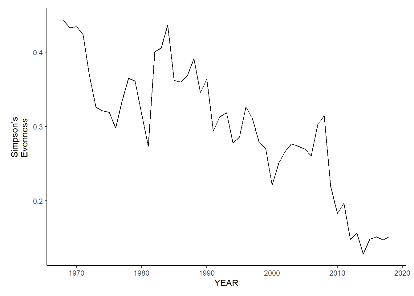

gom_fl_simpson.e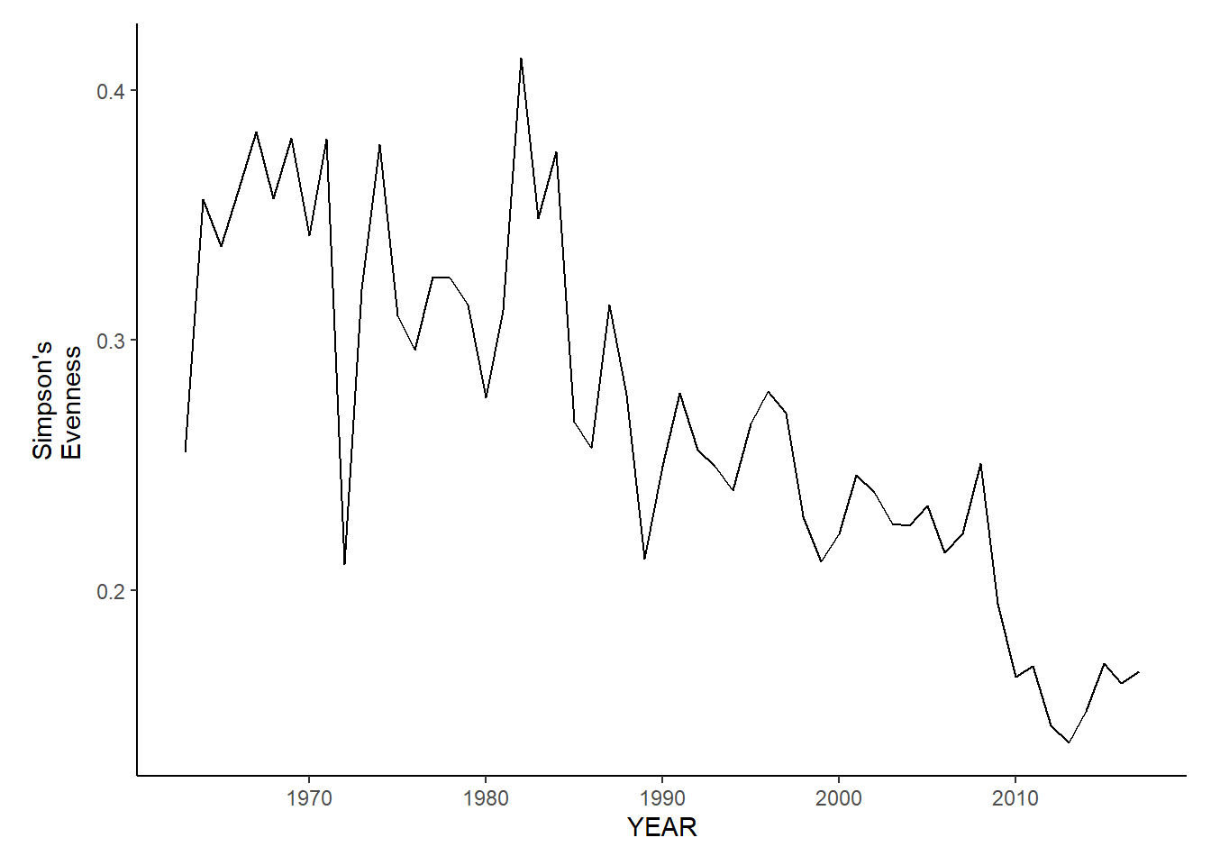

Taxonomic diversity

gom_sp_tax.diversity<-ggplot()+geom_line(data=gom_spring_inds, aes(YEAR, avg_delta))+theme_classic()+ylab(expression(paste("Taxonomic\nDiversity")))+theme(plot.margin = margin(10, 10, 10, 25))
                                   
gom_fl_tax.diversity<-ggplot()+geom_line(data=gom_fall_inds, aes(YEAR, avg_delta))+theme_classic()+ylab(expression(paste("Taxonomic\nDiversity")))+theme(plot.margin = margin(10, 10, 10, 25)) 

gom_sp_tax.diversity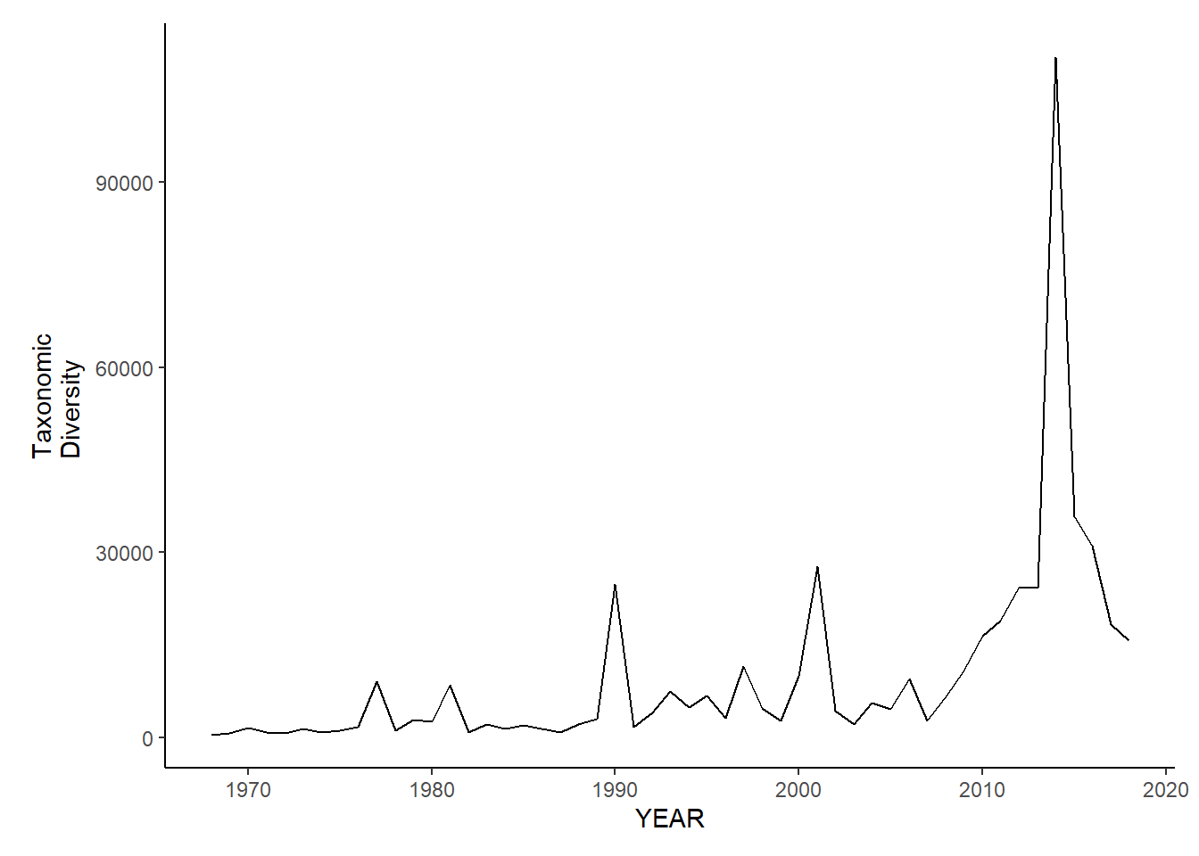

gom_fl_tax.diversity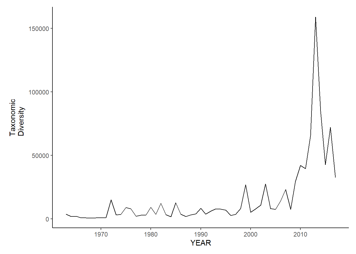

Taxonomic distinctness

gom_sp_tax.distinct<-ggplot()+geom_line(data=gom_spring_inds, aes(YEAR, avg_delta_star))+theme_classic()+ylab(expression(paste("Taxonomic\nDistinctness")))+theme(plot.margin = margin(10, 10, 10, 25))
                                   
gom_fl_tax.distinct<-ggplot()+geom_line(data=gom_fall_inds, aes(YEAR, avg_delta_star))+theme_classic()+ylab(expression(paste("Taxonomic\nDistinctness")))+theme(plot.margin = margin(10, 10, 10, 25)) 

gom_sp_tax.distinct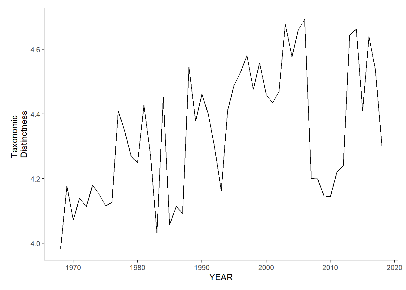

gom_fl_tax.distinct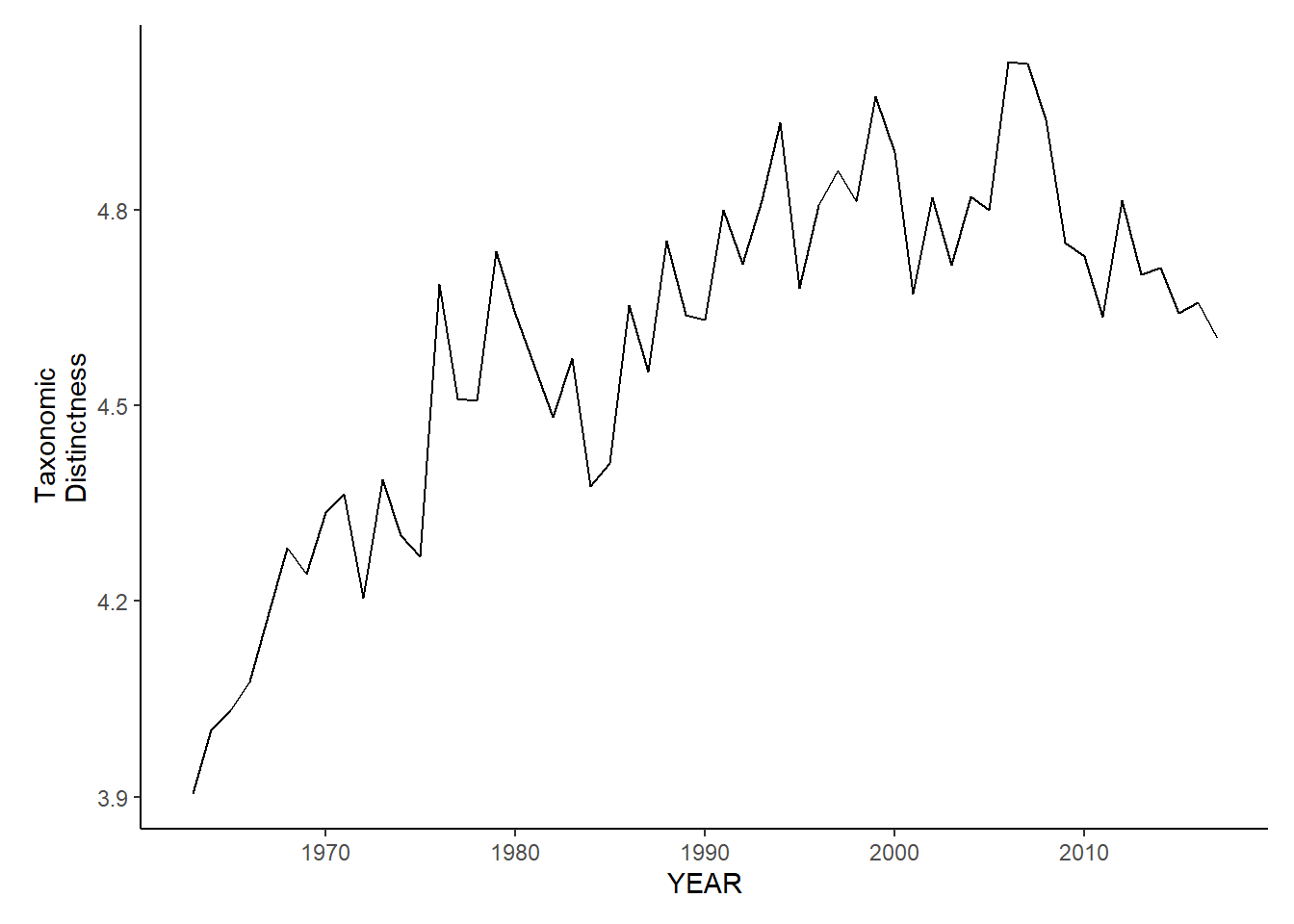

Average taxonomic distinctness

gom_sp_avg.tax.distinct<-ggplot()+geom_line(data=gom_spring_inds, aes(YEAR, avg_delta_plus))+theme_classic()+ylab(expression(paste("Average\nTaxonomic\nDistinctness")))+theme(plot.margin = margin(10, 10, 10, 25))
                                   
gom_fl_avg.tax.distinct<-ggplot()+geom_line(data=gom_fall_inds, aes(YEAR, avg_delta_plus))+theme_classic()+ylab(expression(paste("Average\nTaxonomic\nDistinctness")))+theme(plot.margin = margin(10, 10, 10, 25)) 

gom_sp_avg.tax.distinct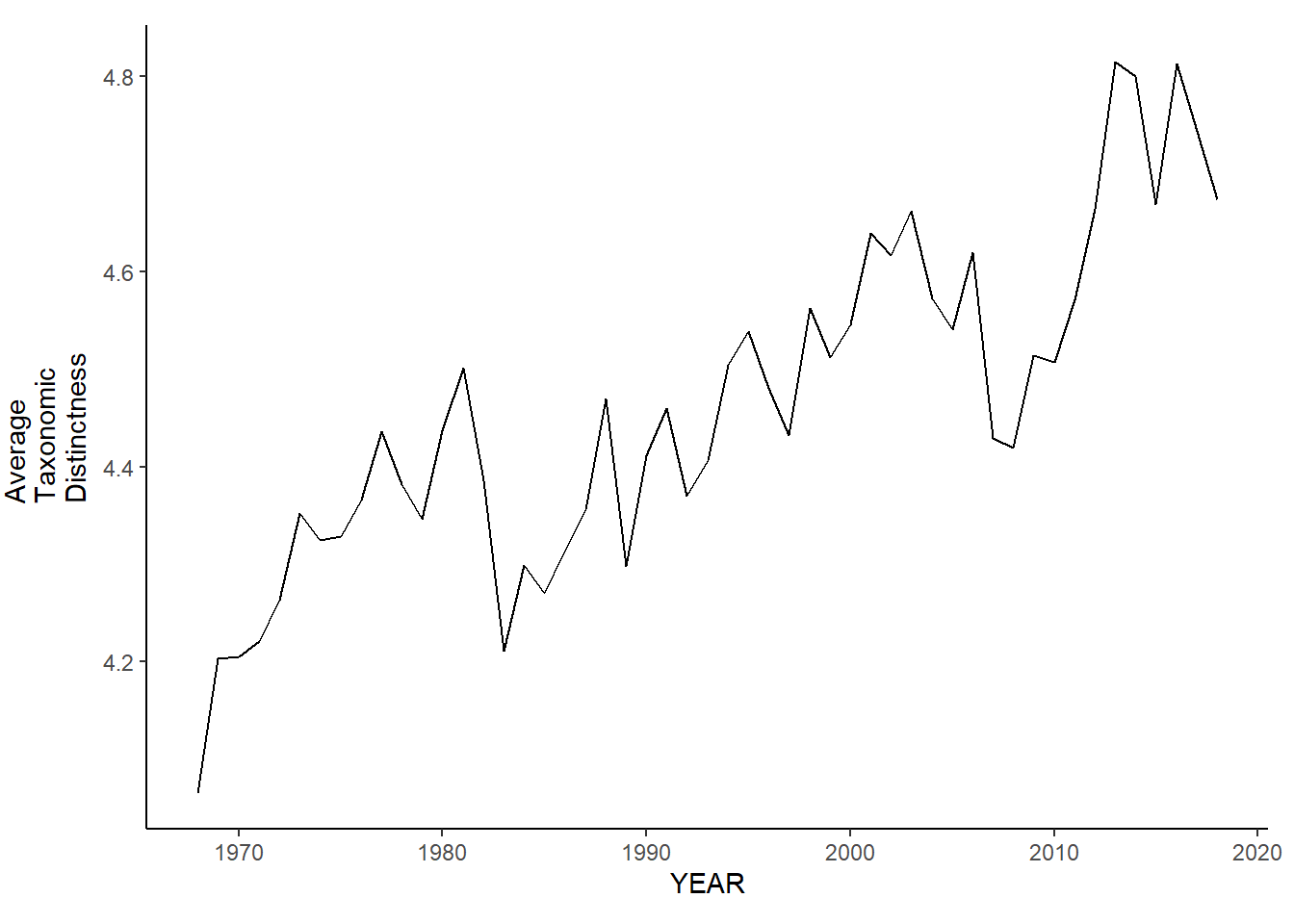

gom_fl_avg.tax.distinct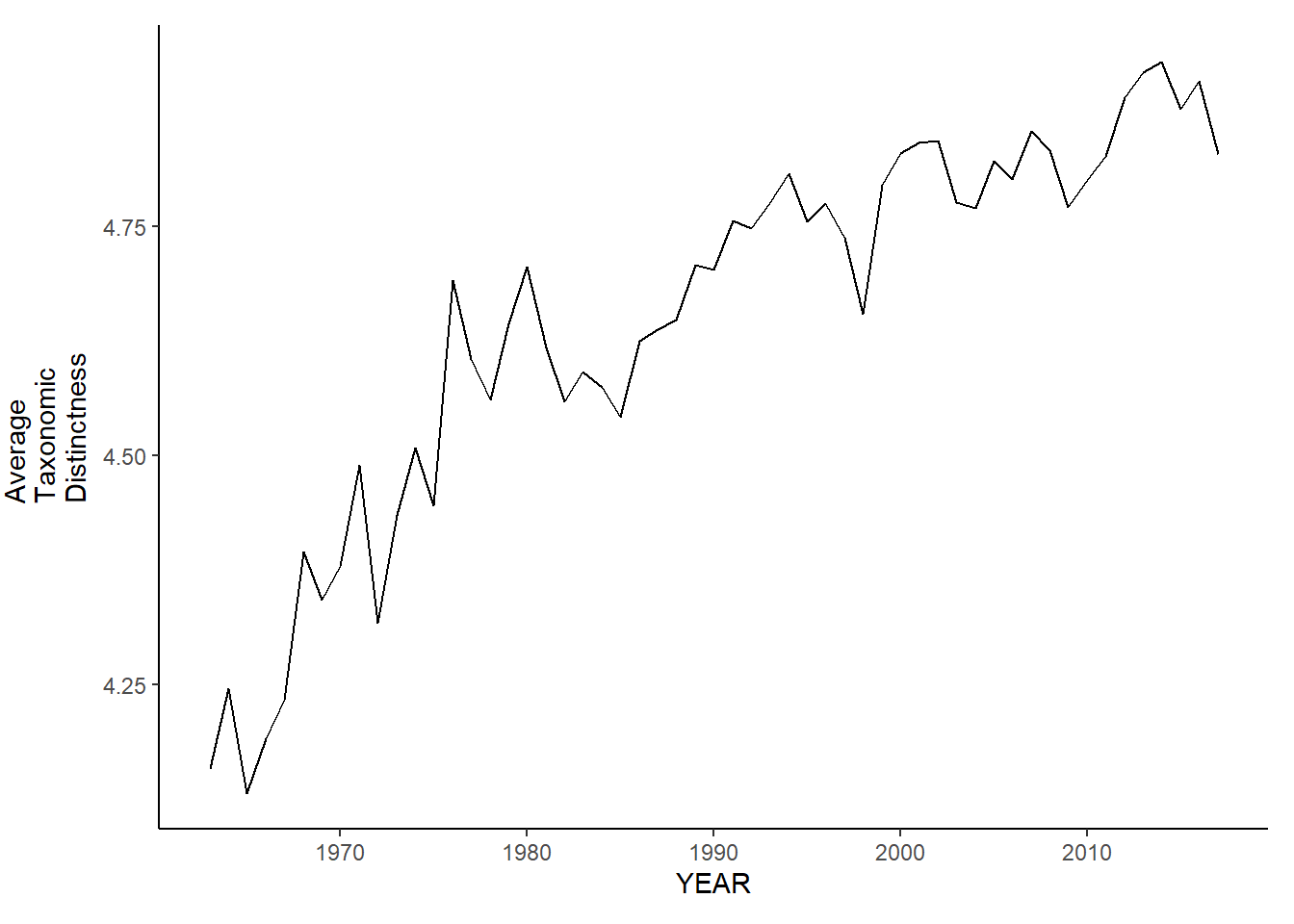

Variation in taxonomic distinctness

gom_sp_var.tax.distinct<-ggplot()+geom_line(data=gom_spring_inds, aes(YEAR, avg_delta_var))+theme_classic()+ylab(expression(paste("Variation\nTaxonomic\nDistinctness")))+theme(plot.margin = margin(10, 10, 10, 25))
                                   
gom_fl_var.tax.distinct<-ggplot()+geom_line(data=gom_fall_inds, aes(YEAR, avg_delta_var))+theme_classic()+ylab(expression(paste("Variation\nTaxonomic\nDistinctness")))+theme(plot.margin = margin(10, 10, 10, 25)) 

gom_sp_var.tax.distinct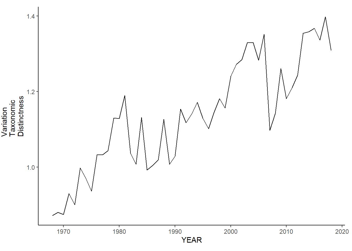

gom_fl_var.tax.distinct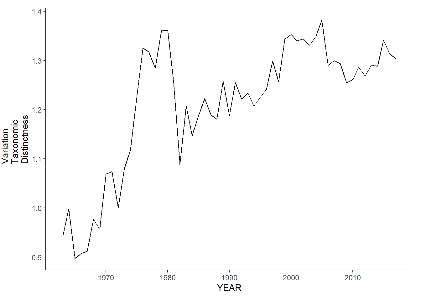

Comparison plots

library(ggthemes)
#combine indices from different surveys
me_inds<-full_join(me_richness,me_shannon )%>%
  full_join(me_simpson)%>%
  full_join(d_season)%>%
  rename(avg_N_species=avg_richness, avg_H_index= avg_shannon, avg_D_index=avg_simpsonD, avg_E_index=avg_simpsonE, YEAR=Year)

me_fall_inds<-filter(me_inds, Season=="Fall")
me_spring_inds<-filter(me_inds, Season=="Spring")

me_fall_inds$Survey<-"ME"
me_spring_inds$Survey<-"ME"

ma_fall_inds$Survey<-"MA"
ma_spring_inds$Survey<-"MA"

nefsc_fall_inds$Survey<-"NEFSC"
nefsc_spring_inds$Survey<-"NEFSC"

gom_fall_inds$Survey<-"GOM"
gom_spring_inds$Survey<-"GOM"

fall_inds<-full_join(me_fall_inds, ma_fall_inds)%>%
  full_join(nefsc_fall_inds)%>%
  full_join(gom_fall_inds)

spring_inds<-full_join(me_spring_inds, ma_spring_inds)%>%
  full_join(nefsc_spring_inds)%>%
  full_join(gom_spring_inds)

#plot
all_rich<-ggplot()+geom_line(data=fall_inds, aes(x=YEAR, y=avg_N_species, color=Survey))+
  scale_color_colorblind()+theme_classic()

all_shannon<-ggplot()+geom_line(data=fall_inds, aes(x=YEAR, y=avg_H_index, color=Survey))+
  scale_color_colorblind()+theme_classic()

all_simpsonD<-ggplot()+geom_line(data=fall_inds, aes(x=YEAR, y=avg_D_index, color=Survey))+
  scale_color_colorblind()+theme_classic()

allSimpsonE<-ggplot()+geom_line(data=fall_inds, aes(x=YEAR, y=avg_E_index, color=Survey))+
  scale_color_colorblind()+theme_classic()

all_taxdiversity<-ggplot()+geom_line(data=fall_inds, aes(x=YEAR, y=avg_delta, color=Survey))+
  scale_color_colorblind()+theme_classic()

all_taxdistinct<-ggplot()+geom_line(data=fall_inds, aes(x=YEAR, y=avg_delta_plus, color=Survey))+
  scale_color_colorblind()+theme_classic()

all_avgtaxdistinct<-ggplot()+geom_line(data=fall_inds, aes(x=YEAR, y=avg_delta_star, color=Survey))+
  scale_color_colorblind()+theme_classic()

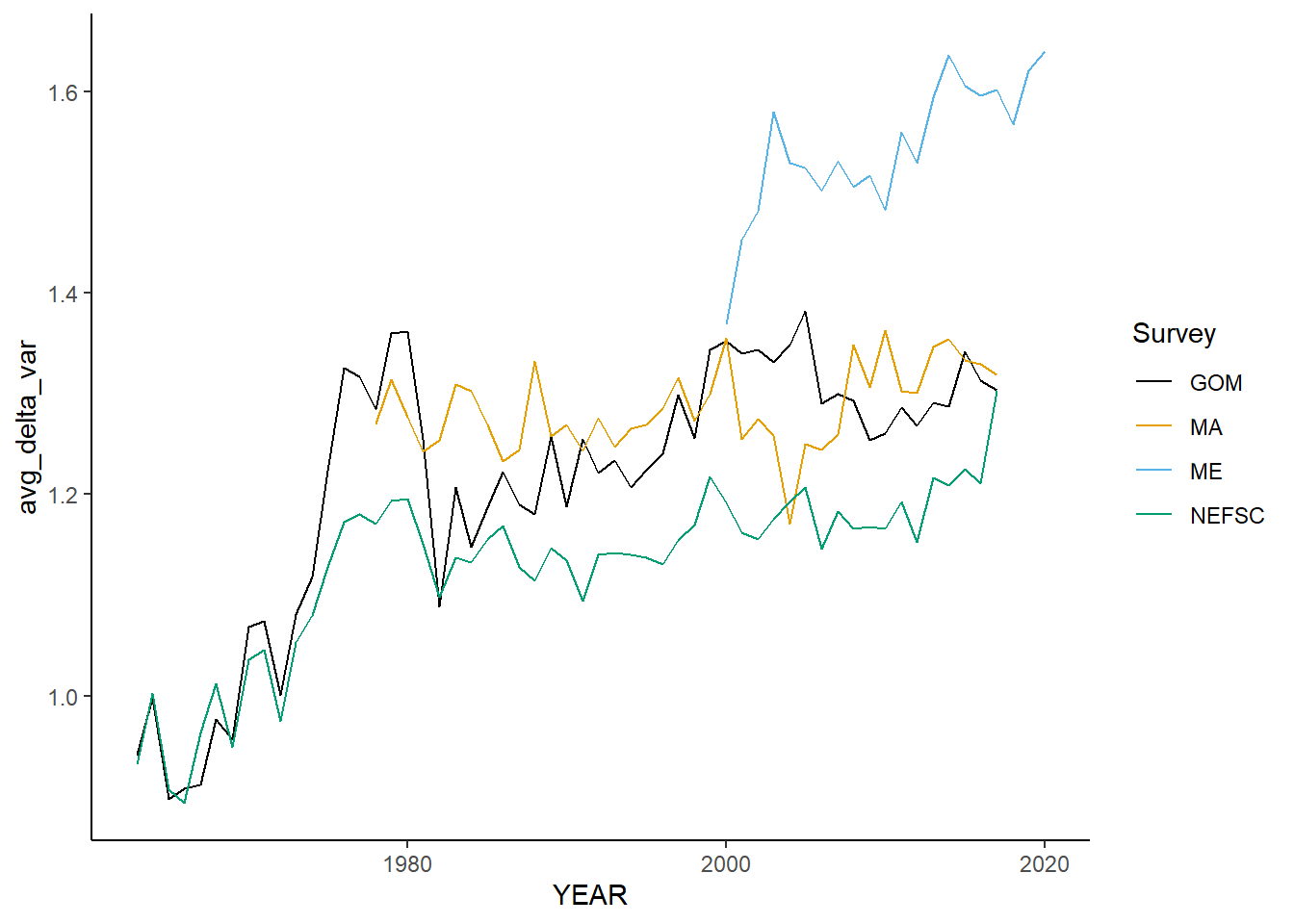
all_vartaxdistinct<-ggplot()+geom_line(data=fall_inds, aes(x=YEAR, y=avg_delta_var, color=Survey))+
  scale_color_colorblind()+theme_classic()

all_rich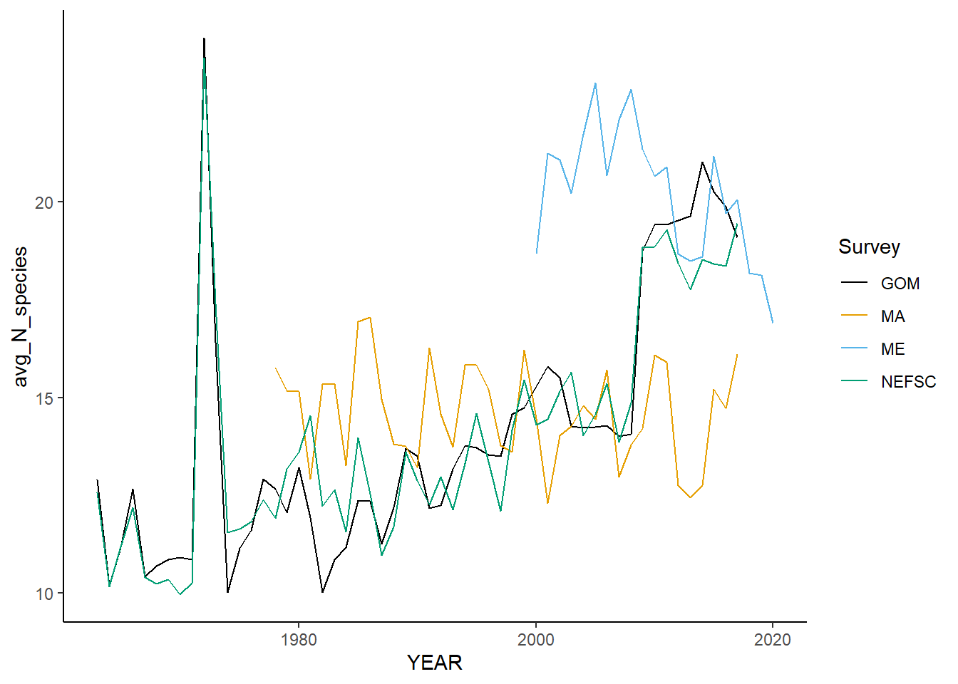

all_shannon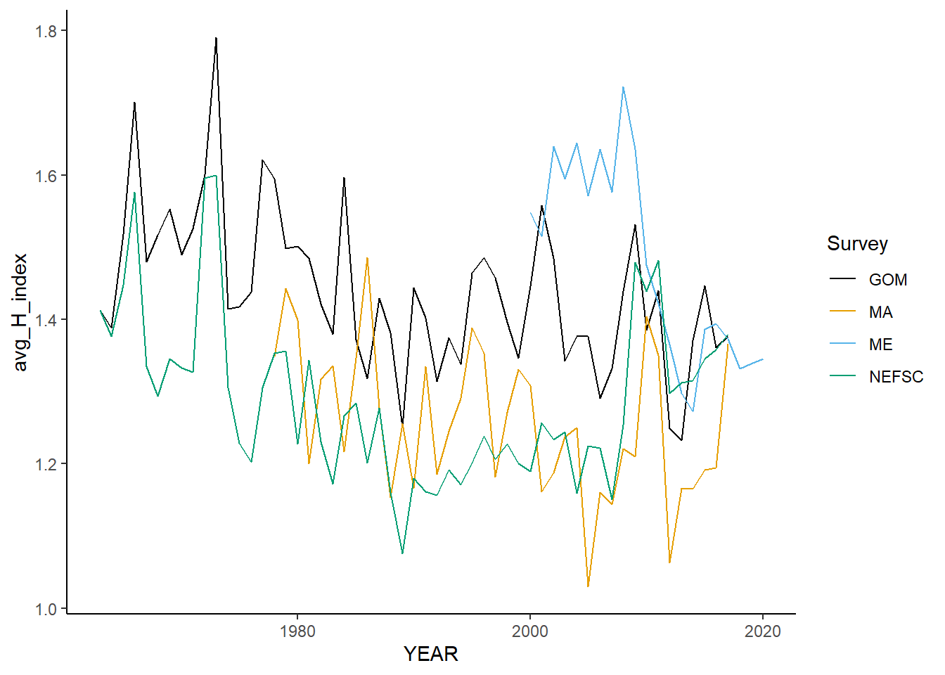

all_simpsonD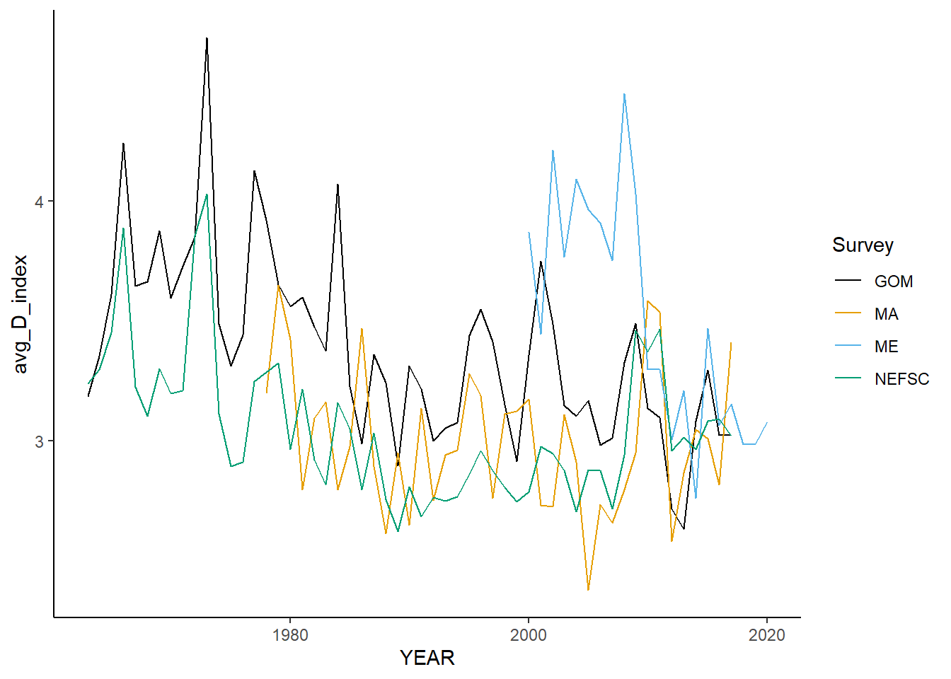

allSimpsonE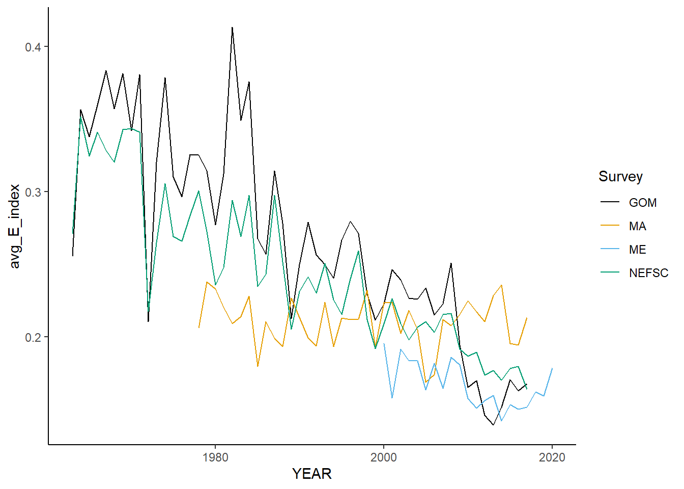

all_taxdiversity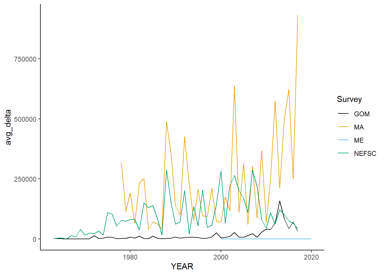

all_taxdistinct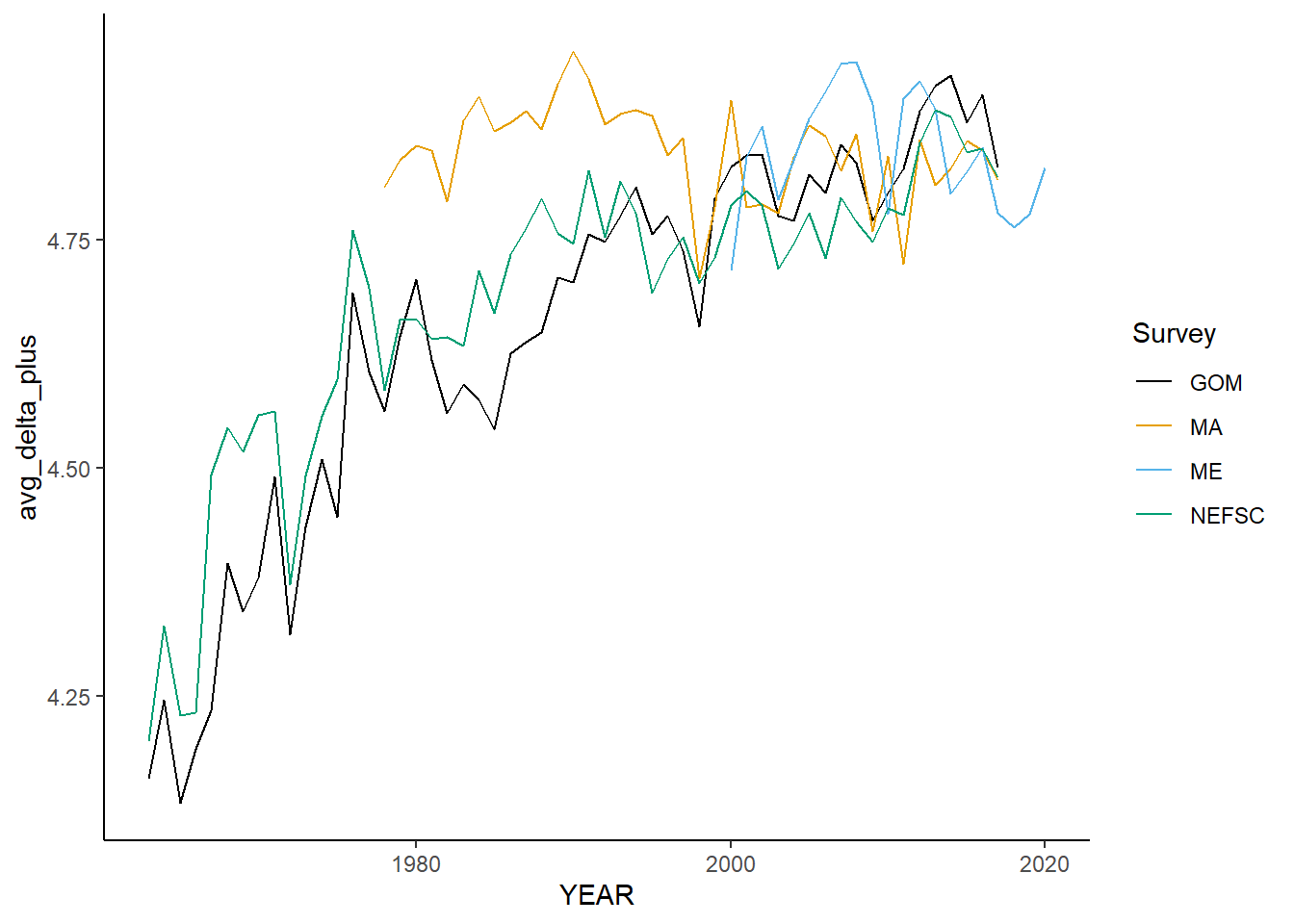

all_avgtaxdistinct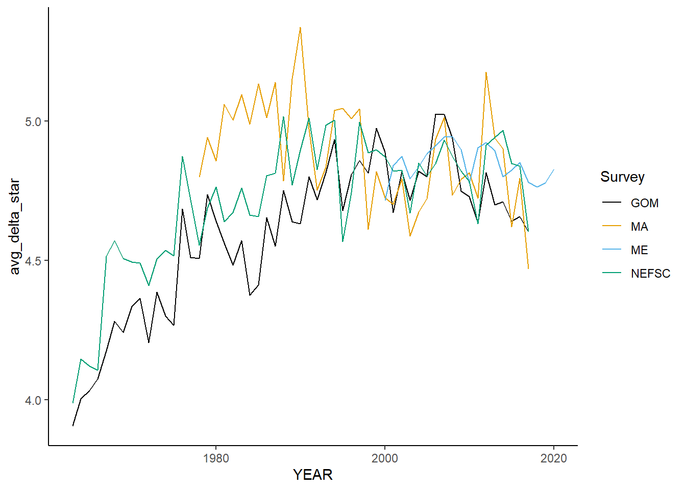

all_vartaxdistinct