Maine-New Hampshire Inshore Trawl

Trawl plots

Top 5 species

#load packages
library(tidyverse)
library(vegan)
library(ggrepel)
library(ggforce)
library(ggnewscale)
library(ggthemes)
library(here)

#read in data (functional groups were added in Biodiversity_metrics_groups.R)
trawl_data<-read.csv(here("Data/ME_trawl_NMDS_data.csv"))[,c(2:17, 20)]
#updated data
trawl_data_update<-read.csv(here("Data/MaineDMR_Trawl_Survey_Catch_Data_2021-05-14.csv"))

cpue_species<-group_by(trawl_data_update,Year,Season)%>%
  mutate(tows=n_distinct(Tow_Number))%>%
  group_by(COMMON_NAME,Year,Season)%>%
  mutate(biomass=sum(Expanded_Weight_kg, na.rm = T),catch=sum(Expanded_Catch, na.rm=T))%>%
  mutate(weight_percent=biomass/tows, catch_percent=catch/tows)%>%
  group_by(Year,COMMON_NAME)%>%
  summarise(weight_prop=mean(weight_percent),catch_prop=mean(catch_percent))


top10<-group_by(cpue_species, COMMON_NAME)%>%
  summarise(mean(weight_prop))
cpue_species$COMMON_NAME[!cpue_species$COMMON_NAME %in% c("lobster american","hake silver (whiting)","herring atlantic","dogfish spiny","alewife")]<-"Other"

ggplot(cpue_species)+
  geom_bar(aes(x=Year, y=weight_prop, fill=COMMON_NAME), position="fill", stat = "identity")+
  labs(x="Year", y="Proportion of Biomass/ tow (kg)", color="Species")+
  scale_fill_colorblind()

  # theme(text=element_text(size=14))+
  # theme(axis.text.y = element_text(colour = "black", size = 16, face = "bold"), 
  #       axis.text.x = element_text(colour = "black", face = "bold", size = 16), 
  #       legend.text = element_text(size = 16, face ="bold", colour ="black"), 
  #       legend.position = "right", axis.title.y = element_text(face = "bold", size = 18), 
  #       axis.title.x = element_text(face = "bold", size = 16, colour = "black"), 
  #       legend.title = element_text(size = 18, colour = "black", face = "bold"), 
  #       panel.background = element_blank(), panel.border = element_rect(colour = "black", fill = NA, size = 0.5),
  #       legend.key=element_blank())

ggplot(cpue_species)+
  geom_line(aes(x=Year, y=weight_prop, color=COMMON_NAME, group=COMMON_NAME), size=1)+
  theme_classic()+
  scale_color_colorblind()+
  labs(x="Year", y="biomass/ tow", color="Species")

  #scale_x_discrete(labels =c(seq(2000,2017, by=1)))+
  #theme(text=element_text(size=18))

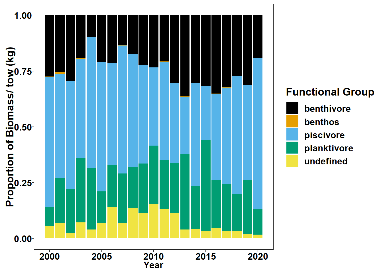
Functional Groups

groups<-read.csv(here("Data/species_groups.csv"))
trawl<-read.csv(here("Data/full_me_dmr_expcatch.csv"))
groups<-full_join(groups,trawl,by="COMMON_NAME")%>%
  select(COMMON_NAME,SCIENTIFIC_NAME,functional_group)%>%
  distinct()


trawl_data<-read.csv(here("Data/MaineDMR_Trawl_Survey_Catch_Data_2021-05-14.csv"))
trawl_3_groups<-left_join(trawl_data, groups, by="COMMON_NAME") #state of the ecosystem groups

trawl_3_groups$functional_group[trawl_3_groups$functional_group==""]<-"undefined"
trawl_3_groups$functional_group[is.na(trawl_3_groups$functional_group)]<-"undefined"

#cpue each year for weight and catch
cpue_year<-group_by(trawl_3_groups,Year,Season)%>%
  mutate(tows=n_distinct(Tow_Number))%>%
  group_by(functional_group,Year,Season)%>%
  mutate(biomass=sum(Expanded_Weight_kg, na.rm = T),catch=sum(Expanded_Catch, na.rm=T))%>%
  mutate(weight_percent=biomass/tows, catch_percent=catch/tows)%>%
  group_by(Year,functional_group)%>%
  summarise(weight_prop=mean(weight_percent),catch_prop=mean(catch_percent))

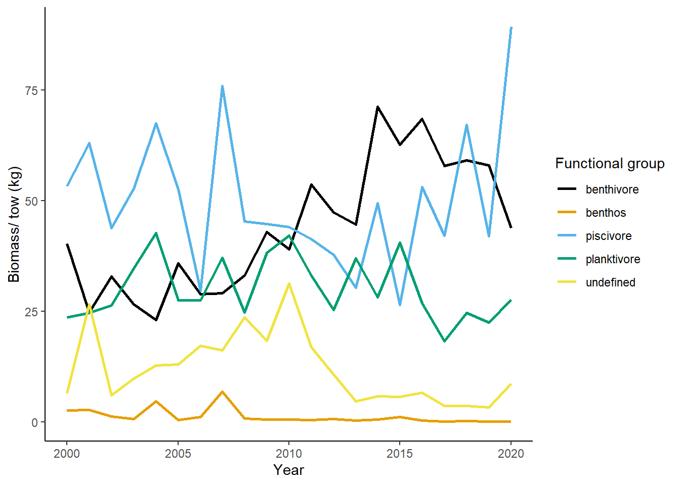
ggplot(cpue_year)+
  geom_line(aes(x=Year, y=weight_prop, color=functional_group, group=functional_group), size=1)+
  theme_classic()+
  scale_color_colorblind()+
  labs(x="Year", y="Biomass/ tow (kg)", color="Functional group")

  #theme(text=element_text(size=14))


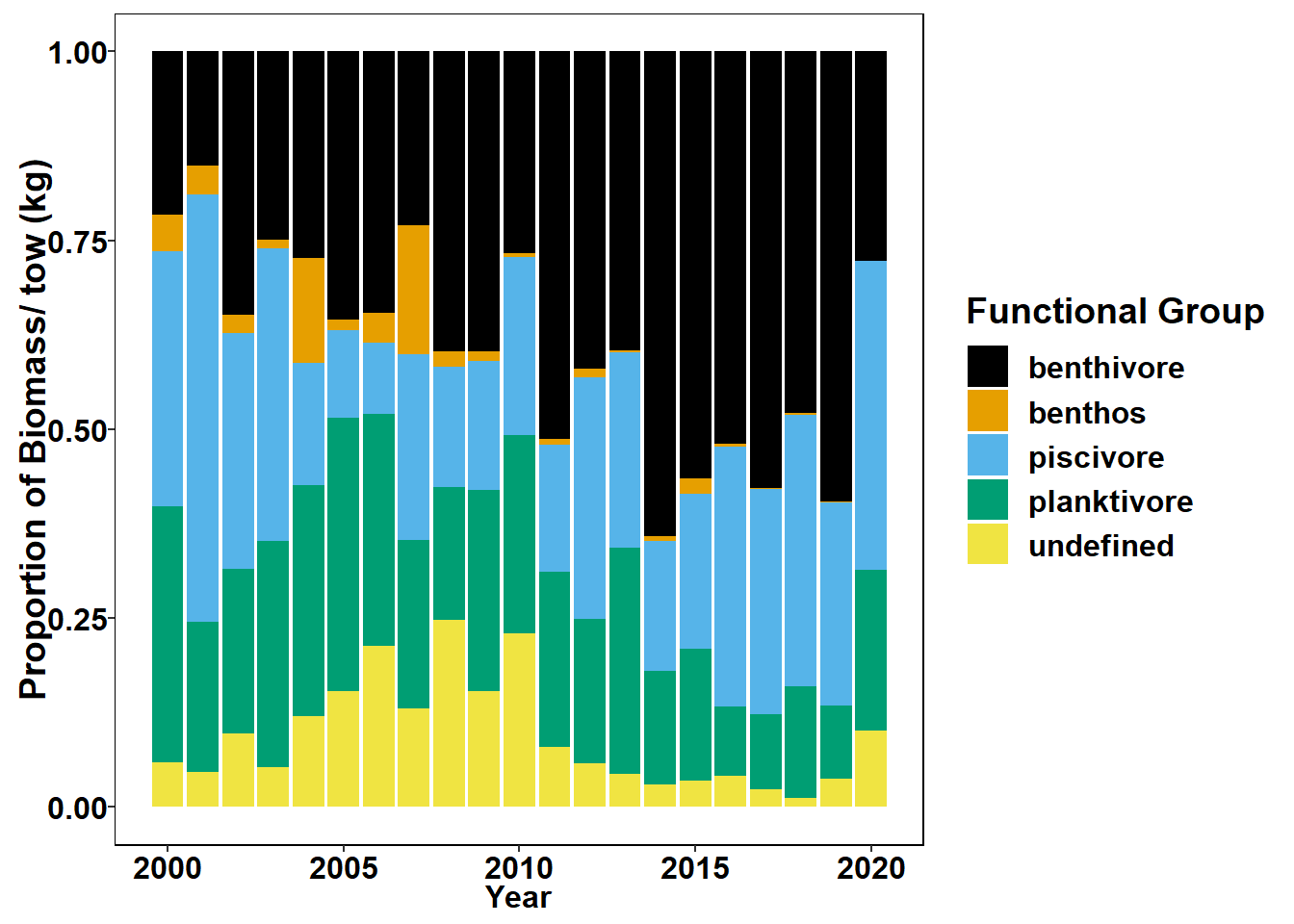
ggplot(cpue_year)+
  geom_bar(aes(x=Year, y=weight_prop, fill=functional_group), position="fill", stat = "identity")+
  scale_fill_colorblind(name="Functional Group")+
  labs(x="Year", y="Proportion of Biomass/ tow (kg)", color="Functional group")

  # theme(text=element_text(size=14))+
  # theme(axis.text.y = element_text(colour = "black", size = 16, face = "bold"), 
  #       axis.text.x = element_text(colour = "black", face = "bold", size = 16), 
  #       legend.text = element_text(size = 16, face ="bold", colour ="black"), 
  #       legend.position = "right", axis.title.y = element_text(face = "bold", size = 18), 
  #       axis.title.x = element_text(face = "bold", size = 16, colour = "black"), 
  #       legend.title = element_text(size = 18, colour = "black", face = "bold"), 
  #       panel.background = element_blank(), panel.border = element_rect(colour = "black", fill = NA, size = 0.5),
  #       legend.key=element_blank())


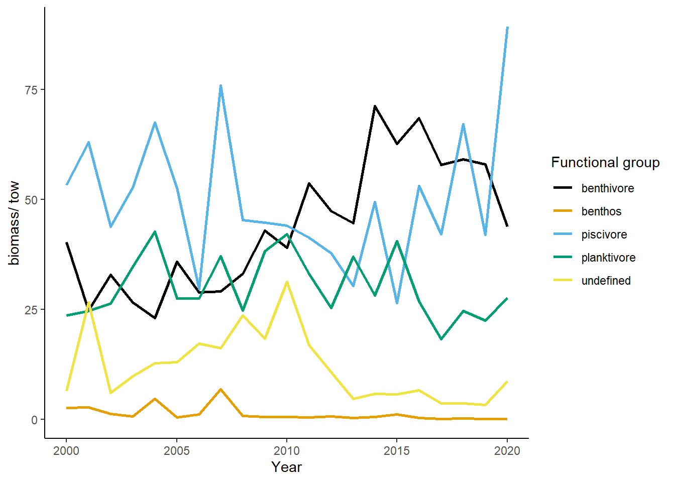
ggplot(cpue_year)+
  geom_line(aes(x=Year, y=weight_prop, color=functional_group, group=functional_group), size=1)+
  theme_classic()+
  scale_color_colorblind()+
  labs(x="Year", y="biomass/ tow", color="Functional group")

  #scale_x_discrete(labels =c(seq(2000,2017, by=1)))+
  #theme(text=element_text(size=16))

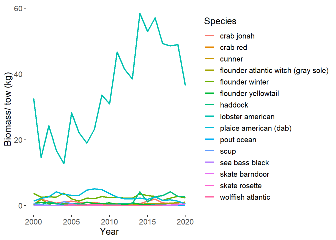
Benthivore

####Each functional group####
benthivore<-filter(trawl_3_groups, functional_group=="benthivore")
cpue_benthivore<-group_by(benthivore,Year,Season)%>%
  mutate(tows=n_distinct(Tow_Number))%>%
  group_by(COMMON_NAME,Year,Season)%>%
  mutate(biomass=sum(Expanded_Weight_kg, na.rm = T),catch=sum(Expanded_Catch, na.rm=T))%>%
  mutate(weight_percent=biomass/tows, catch_percent=catch/tows)%>%
  group_by(Year,COMMON_NAME)%>%
  summarise(weight_prop=mean(weight_percent),catch_prop=mean(catch_percent))

ggplot(cpue_benthivore)+
  geom_line(aes(x=Year, y=weight_prop, color=COMMON_NAME, group=COMMON_NAME), size=1)+
  theme_classic()+
  labs(x="Year", y="Biomass/ tow (kg)", color="Species")+
  theme(text=element_text(size=14))

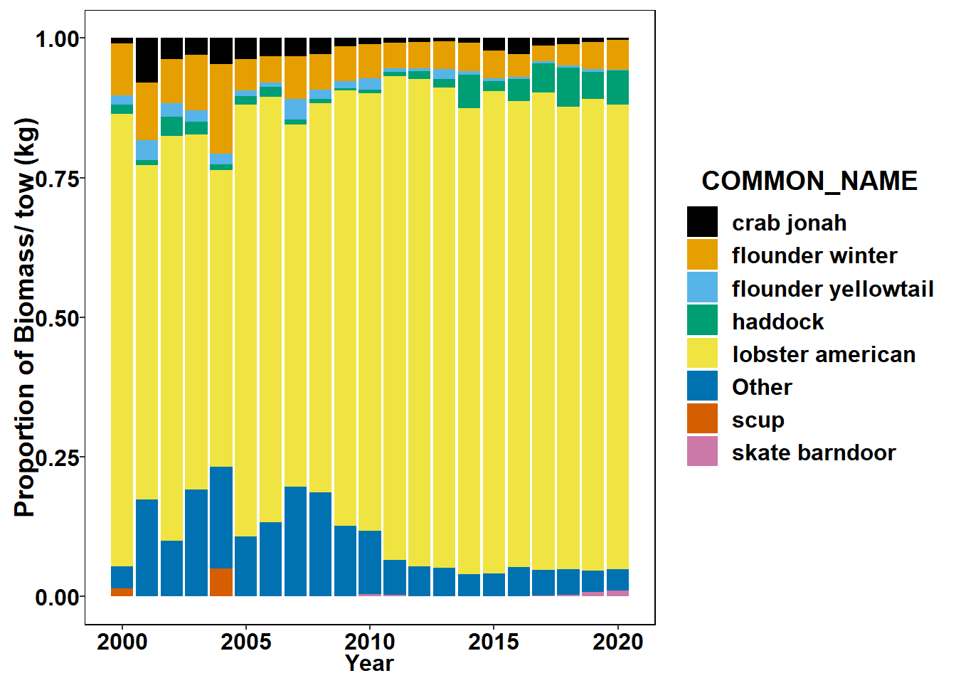
top10<-group_by(cpue_benthivore, COMMON_NAME)%>%
  summarise(mean(weight_prop))
cpue_benthivore$COMMON_NAME[!cpue_benthivore$COMMON_NAME %in% c("lobster american","american plaice (dab)","flounder winter","haddock","crab jonah","flounder atlantic witch (grey sole)","flounder yellowtail","scup","skate barndoor")]<-"Other"

ggplot(cpue_benthivore)+
  geom_bar(aes(x=Year, y=weight_prop, fill=COMMON_NAME), position="fill", stat = "identity")+
  labs(x="Year", y="Proportion of Biomass/ tow (kg)", color="Species")+
  scale_fill_colorblind()

  # theme(text=element_text(size=14))+
  # theme(axis.text.y = element_text(colour = "black", size = 16, face = "bold"), 
  #       axis.text.x = element_text(colour = "black", face = "bold", size =16), 
  #       legend.text = element_text(size = 16, face ="bold", colour ="black"), 
  #       legend.position = "right", axis.title.y = element_text(face = "bold", size = 18), 
  #       axis.title.x = element_text(face = "bold", size = 16, colour = "black"), 
  #       legend.title = element_text(size = 18, colour = "black", face = "bold"), 
  #       panel.background = element_blank(), panel.border = element_rect(colour = "black", fill = NA, size = 0.5),
  #       legend.key=element_blank())

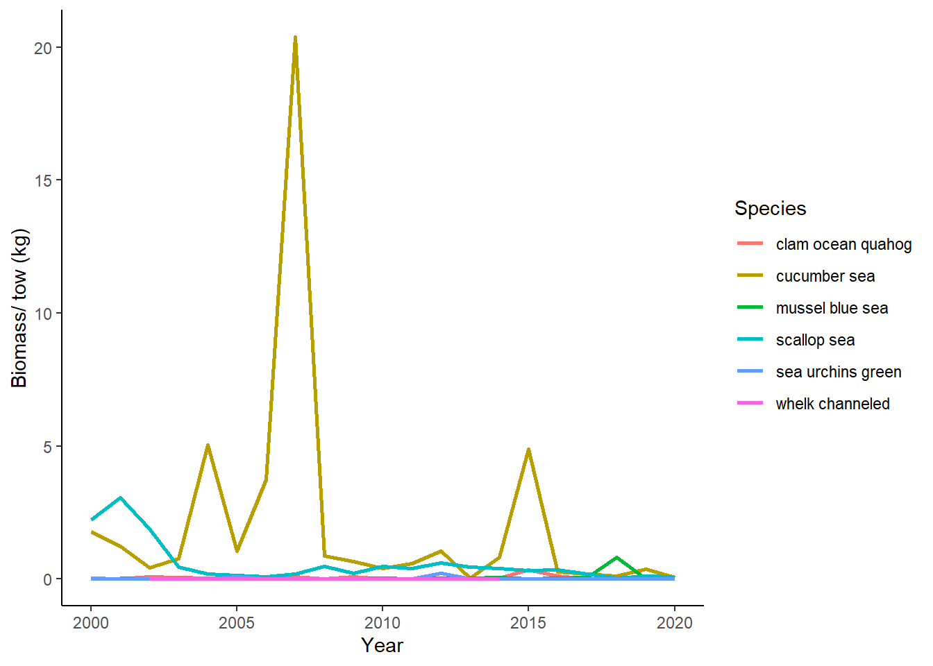
Benthos

benthos<-filter(trawl_3_groups, functional_group=="benthos")
cpue_benthos<-group_by(benthos,Year,Season)%>%
  mutate(tows=n_distinct(Tow_Number))%>%
  group_by(COMMON_NAME,Year,Season)%>%
  mutate(biomass=sum(Expanded_Weight_kg, na.rm = T),catch=sum(Expanded_Catch, na.rm=T))%>%
  mutate(weight_percent=biomass/tows, catch_percent=catch/tows)%>%
  group_by(Year,COMMON_NAME)%>%
  summarise(weight_prop=mean(weight_percent),catch_prop=mean(catch_percent))

ggplot(cpue_benthos)+
  geom_line(aes(x=Year, y=weight_prop, color=COMMON_NAME, group=COMMON_NAME), size=1)+
  theme_classic()+
  labs(x="Year", y="Biomass/ tow (kg)", color="Species")

  #theme(text=element_text(size=20))

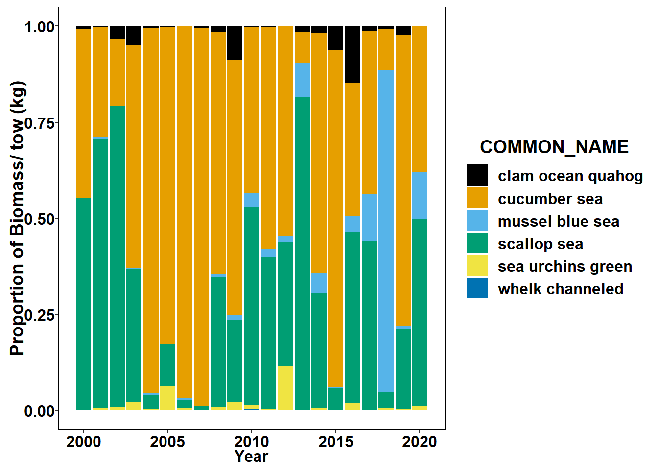
top10<-group_by(cpue_benthos, COMMON_NAME)%>%
  summarise(mean(weight_prop))

ggplot(cpue_benthos)+
  geom_bar(aes(x=Year, y=weight_prop, fill=COMMON_NAME), position="fill", stat = "identity")+
  labs(x="Year", y="Proportion of Biomass/ tow (kg)", color="Species")+
  scale_fill_colorblind()

  # theme(text=element_text(size=14))+
  # theme(axis.text.y = element_text(colour = "black", size = 16, face = "bold"), 
  #       axis.text.x = element_text(colour = "black", face = "bold", size = 16), 
  #       legend.text = element_text(size = 16, face ="bold", colour ="black"), 
  #       legend.position = "right", axis.title.y = element_text(face = "bold", size = 18), 
  #       axis.title.x = element_text(face = "bold", size = 16, colour = "black"), 
  #       legend.title = element_text(size = 18, colour = "black", face = "bold"), 
  #       panel.background = element_blank(), panel.border = element_rect(colour = "black", fill = NA, size = 0.5),
  #       legend.key=element_blank())

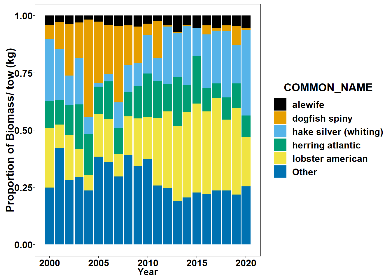
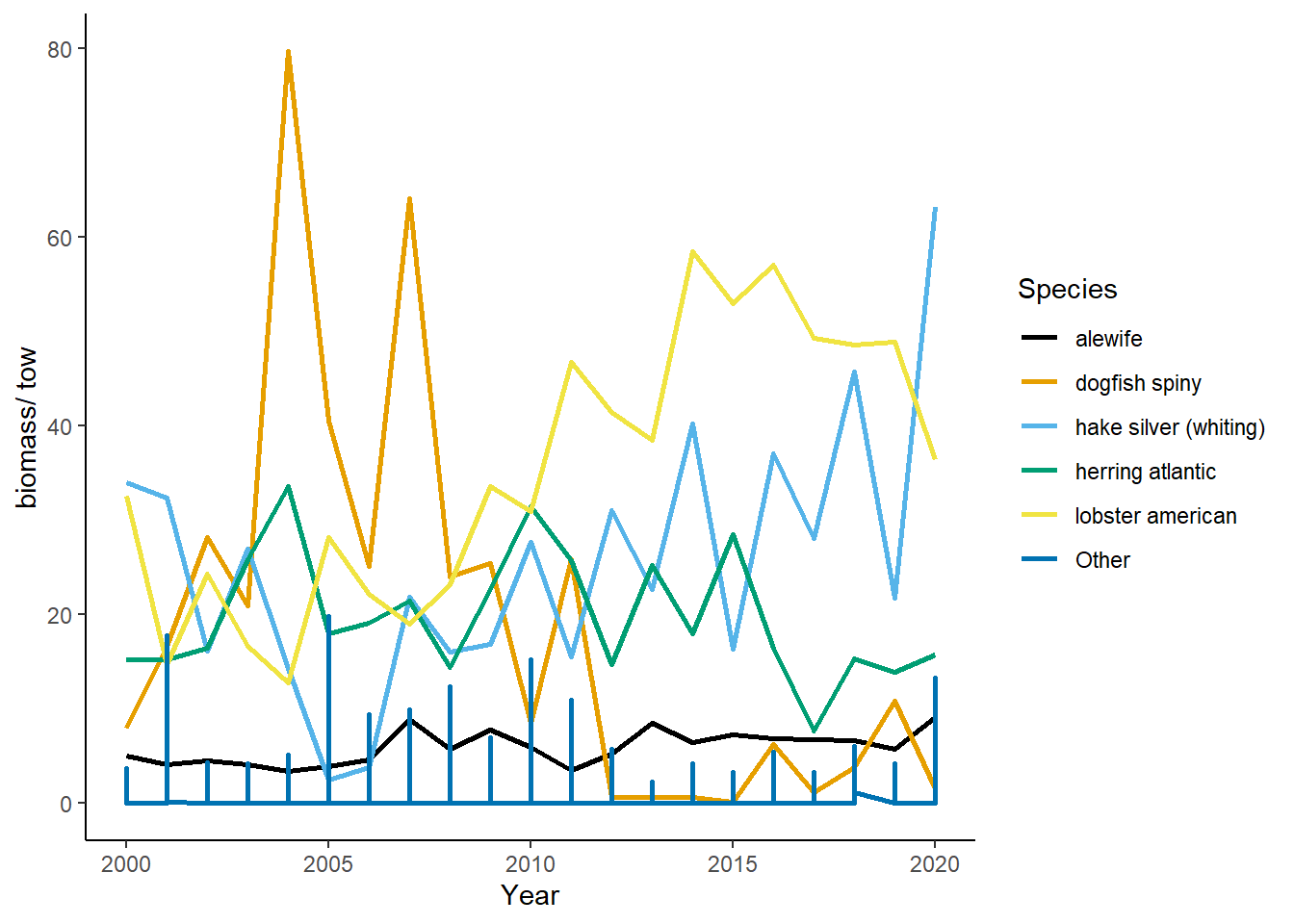
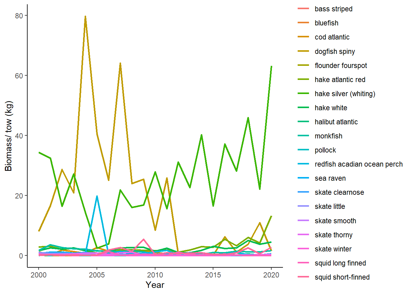
Piscivore

piscivore<-filter(trawl_3_groups, functional_group=="piscivore")
cpue_piscivore<-group_by(piscivore,Year,Season)%>%
  mutate(tows=n_distinct(Tow_Number))%>%
  group_by(COMMON_NAME,Year,Season)%>%
  mutate(biomass=sum(Expanded_Weight_kg, na.rm = T),catch=sum(Expanded_Catch, na.rm=T))%>%
  mutate(weight_percent=biomass/tows, catch_percent=catch/tows)%>%
  group_by(Year,COMMON_NAME)%>%
  summarise(weight_prop=mean(weight_percent),catch_prop=mean(catch_percent))

ggplot(cpue_piscivore)+
  geom_line(aes(x=Year, y=weight_prop, color=COMMON_NAME, group=COMMON_NAME), size=1)+
  theme_classic()+
  labs(x="Year", y="Biomass/ tow (kg)", color="Species")

  #theme(text=element_text(size=20))


top10<-group_by(cpue_piscivore, COMMON_NAME)%>%
  summarise(sum(weight_prop))
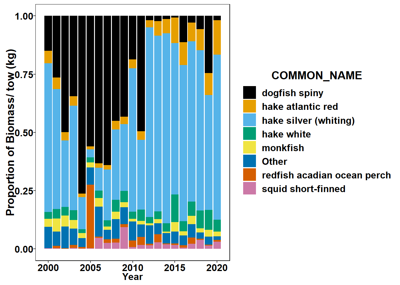
cpue_piscivore$COMMON_NAME[!cpue_piscivore$COMMON_NAME %in% c("hake silver (whiting)","dogfish spiny","hake atlantic red","hake white","redfish acadian ocean perch","monkfish","squid short-finned")]<-"Other"

ggplot(cpue_piscivore)+
  geom_bar(aes(x=Year, y=weight_prop, fill=COMMON_NAME), position="fill", stat = "identity")+
  labs(x="Year", y="Proportion of Biomass/ tow (kg)", color="Species")+
  scale_fill_colorblind()

  # theme(text=element_text(size=14))+
  # theme(axis.text.y = element_text(colour = "black", size = 16, face = "bold"), 
  #       axis.text.x = element_text(colour = "black", face = "bold", size = 16), 
  #       legend.text = element_text(size = 16, face ="bold", colour ="black"), 
  #       legend.position = "right", axis.title.y = element_text(face = "bold", size = 18), 
  #       axis.title.x = element_text(face = "bold", size = 16, colour = "black"), 
  #       legend.title = element_text(size = 18, colour = "black", face = "bold"), 
  #       panel.background = element_blank(), panel.border = element_rect(colour = "black", fill = NA, size = 0.5),
  #       legend.key=element_blank())

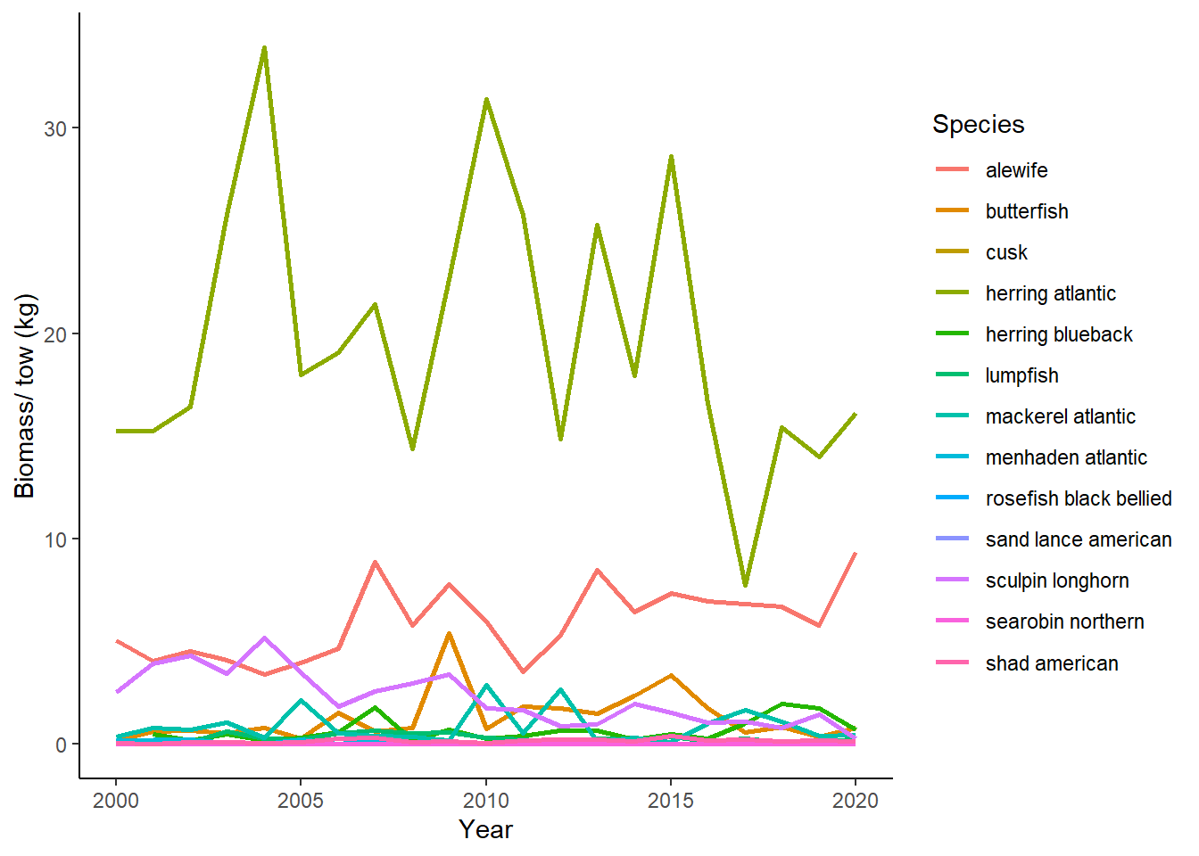
Planktivore

planktivore<-filter(trawl_3_groups, functional_group=="planktivore")
cpue_planktivore<-group_by(planktivore,Year,Season)%>%
  mutate(tows=n_distinct(Tow_Number))%>%
  group_by(COMMON_NAME,Year,Season)%>%
  mutate(biomass=sum(Expanded_Weight_kg, na.rm = T),catch=sum(Expanded_Catch, na.rm=T))%>%
  mutate(weight_percent=biomass/tows, catch_percent=catch/tows)%>%
  group_by(Year,COMMON_NAME)%>%
  summarise(weight_prop=mean(weight_percent),catch_prop=mean(catch_percent))

ggplot(cpue_planktivore)+
  geom_line(aes(x=Year, y=weight_prop, color=COMMON_NAME, group=COMMON_NAME), size=1)+
  theme_classic()+
  labs(x="Year", y="Biomass/ tow (kg)", color="Species")

  #theme(text=element_text(size=20))

top10<-group_by(cpue_planktivore, COMMON_NAME)%>%
  summarise(sum(weight_prop))
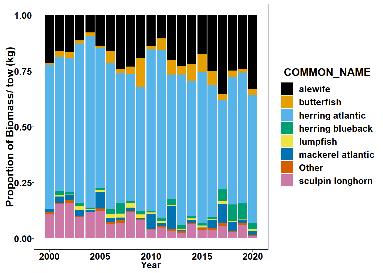
cpue_planktivore$COMMON_NAME[!cpue_planktivore$COMMON_NAME %in% c("herring atlantic","alewife","sculpin longhorn","butterfish","mackerel atlantic","herring blueback","lumpfish")]<-"Other"

ggplot(cpue_planktivore)+
  geom_bar(aes(x=Year, y=weight_prop, fill=COMMON_NAME), position="fill", stat = "identity")+
  labs(x="Year", y="Proportion of Biomass/ tow (kg)", color="Species")+
  scale_fill_colorblind()

  # theme(text=element_text(size=14))+
  # theme(axis.text.y = element_text(colour = "black", size = 16, face = "bold"), 
  #       axis.text.x = element_text(colour = "black", face = "bold", size = 16), 
  #       legend.text = element_text(size = 16, face ="bold", colour ="black"), 
  #       legend.position = "right", axis.title.y = element_text(face = "bold", size = 18), 
  #       axis.title.x = element_text(face = "bold", size = 16, colour = "black"), 
  #       legend.title = element_text(size = 18, colour = "black", face = "bold"), 
  #       panel.background = element_blank(), panel.border = element_rect(colour = "black", fill = NA, size = 0.5),
  #       legend.key=element_blank())

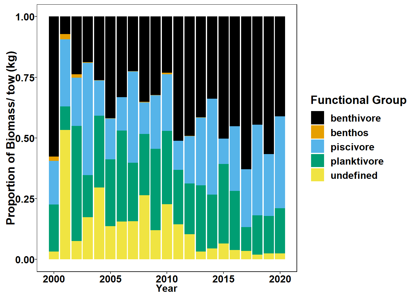
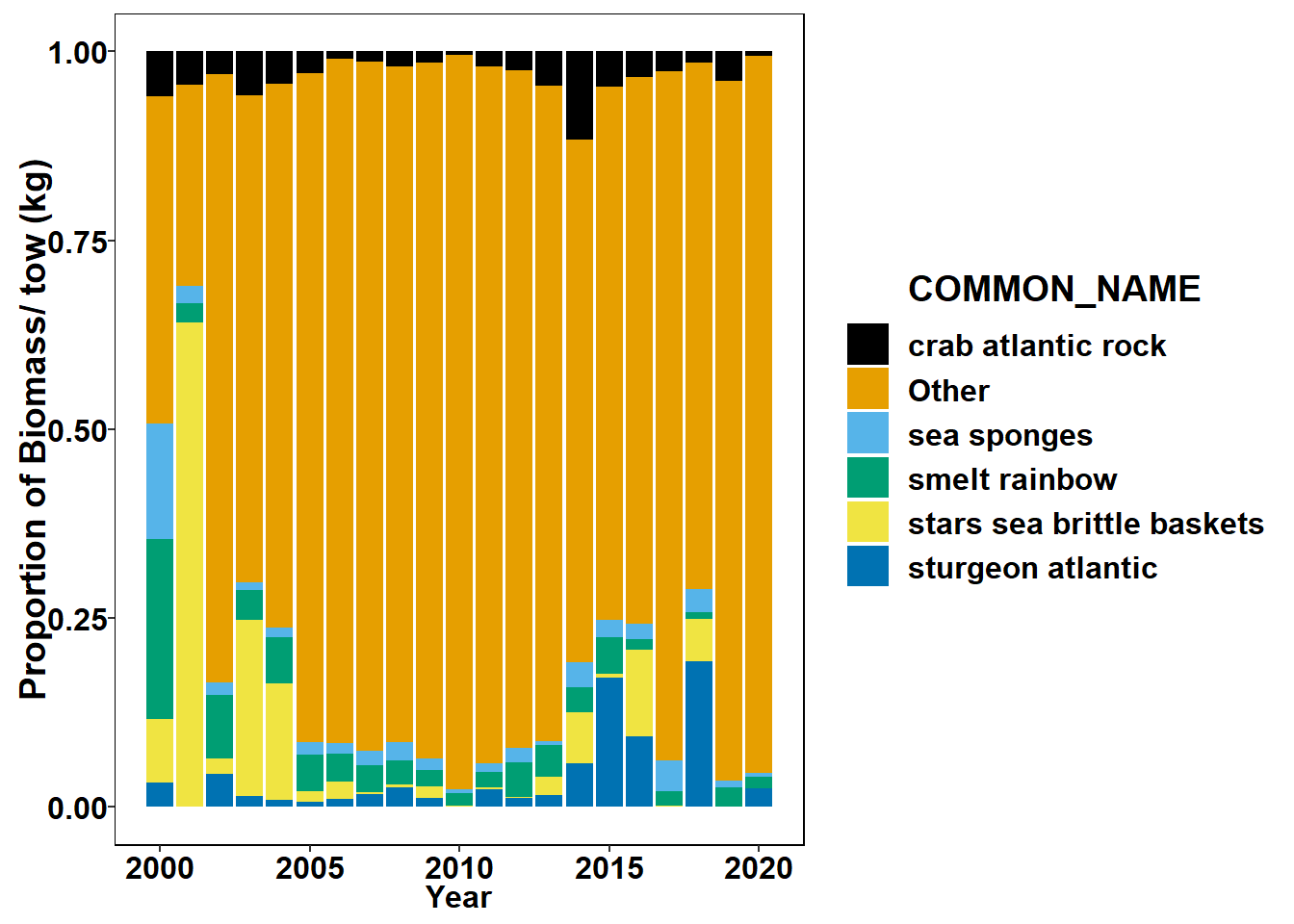
Undefined

undefined<-filter(trawl_3_groups, functional_group=="undefined")
cpue_undefined<-group_by(undefined,Year,Season)%>%
  mutate(tows=n_distinct(Tow_Number))%>%
  group_by(COMMON_NAME,Year,Season)%>%
  mutate(biomass=sum(Expanded_Weight_kg, na.rm = T),catch=sum(Expanded_Catch, na.rm=T))%>%
  mutate(weight_percent=biomass/tows, catch_percent=catch/tows)%>%
  group_by(Year,COMMON_NAME)%>%
  summarise(weight_prop=mean(weight_percent),catch_prop=mean(catch_percent))

paged_table(cpue_undefined)

top10<-group_by(cpue_undefined, COMMON_NAME)%>%
  summarise(sum(weight_prop))
cpue_undefined$COMMON_NAME[!cpue_undefined$COMMON_NAME %in% c("monkfish","stars sea brittle baskets","smelt rainbow","crab atlantic rock","sturgeon atlantic","sea sponges", "waved astrate")]<-"Other"

ggplot(cpue_undefined)+
  geom_bar(aes(x=Year, y=weight_prop, fill=COMMON_NAME), position="fill", stat = "identity")+
  labs(x="Year", y="Proportion of Biomass/ tow (kg)", color="Species")+
  scale_fill_colorblind()

  # theme(text=element_text(size=14))+
  # theme(axis.text.y = element_text(colour = "black", size = 16, face = "bold"), 
  #       axis.text.x = element_text(colour = "black", face = "bold", size = 16), 
  #       legend.text = element_text(size = 16, face ="bold", colour ="black"), 
  #       legend.position = "right", axis.title.y = element_text(face = "bold", size = 18), 
  #       axis.title.x = element_text(face = "bold", size = 16, colour = "black"), 
  #       legend.title = element_text(size = 18, colour = "black", face = "bold"), 
  #       panel.background = element_blank(), panel.border = element_rect(colour = "black", fill = NA, size = 0.5),
  #       legend.key=element_blank())

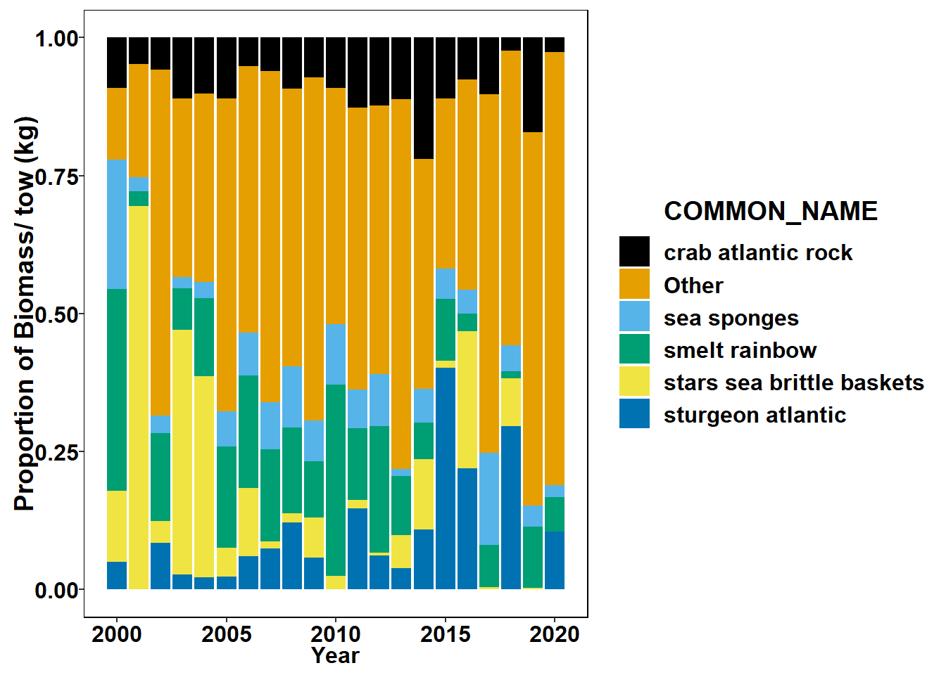
No shrimp

#no shrimp
no_shrimp<-filter(trawl_3_groups, functional_group=="undefined")%>%
  filter(!COMMON_NAME  %in% c("shrimp northern","shrimp montagui","shrimp","shrimp dichelo"))

cpue_no_shrimp<-group_by(no_shrimp,Year,Season)%>%
  mutate(tows=n_distinct(Tow_Number))%>%
  group_by(COMMON_NAME,Year,Season)%>%
  mutate(biomass=sum(Expanded_Weight_kg, na.rm = T),catch=sum(Expanded_Catch, na.rm=T))%>%
  mutate(weight_percent=biomass/tows, catch_percent=catch/tows)%>%
  group_by(Year,COMMON_NAME)%>%
  summarise(weight_prop=mean(weight_percent),catch_prop=mean(catch_percent))

cpue_no_shrimp$COMMON_NAME[!cpue_no_shrimp$COMMON_NAME %in% c("monkfish","stars sea brittle baskets","smelt rainbow","crab atlantic rock","sturgeon atlantic","sea sponges", "waved astrate")]<-"Other"

ggplot(cpue_no_shrimp)+
  geom_bar(aes(x=Year, y=weight_prop, fill=COMMON_NAME), position="fill", stat = "identity")+
  labs(x="Year", y="Proportion of Biomass/ tow (kg)", color="Species")+
  scale_fill_colorblind()

  # theme(text=element_text(size=14))+
  # theme(axis.text.y = element_text(colour = "black", size = 16, face = "bold"), 
  #       axis.text.x = element_text(colour = "black", face = "bold", size = 16), 
  #       legend.text = element_text(size = 16, face ="bold", colour ="black"), 
  #       legend.position = "right", axis.title.y = element_text(face = "bold", size = 18), 
  #       axis.title.x = element_text(face = "bold", size = 16, colour = "black"), 
  #       legend.title = element_text(size = 18, colour = "black", face = "bold"), 
  #       panel.background = element_blank(), panel.border = element_rect(colour = "black", fill = NA, size = 0.5),
  #       legend.key=element_blank())

Regional functional groups

West of the Penobscot

trawl_3_groups$group[trawl_3_groups$Region==1]<-"West"
trawl_3_groups$group[trawl_3_groups$Region==2]<-"West"
trawl_3_groups$group[trawl_3_groups$Region==3]<-"Penobscot"
trawl_3_groups$group[trawl_3_groups$Region==4]<-"East"
trawl_3_groups$group[trawl_3_groups$Region==5]<-"East"

west_groups<-filter(trawl_3_groups, group=="West")

#cpue each year for weight and catch
cpue_year_west<-group_by(west_groups,Year,Season)%>%
  mutate(tows=n_distinct(Tow_Number))%>%
  group_by(functional_group,Year,Season)%>%
  mutate(biomass=sum(Expanded_Weight_kg, na.rm = T),catch=sum(Expanded_Catch, na.rm=T))%>%
  mutate(weight_percent=biomass/tows, catch_percent=catch/tows)%>%
  group_by(Year,functional_group)%>%
  summarise(weight_prop=mean(weight_percent),catch_prop=mean(catch_percent))

ggplot(cpue_year_west)+
  geom_bar(aes(x=Year, y=weight_prop, fill=functional_group), position="fill", stat = "identity")+
  scale_fill_colorblind(name="Functional Group")+
  labs(x="Year", y="Proportion of Biomass/ tow (kg)", color="Functional group")

Penobscot

pen_groups<-filter(trawl_3_groups, group=="Penobscot")

#cpue each year for weight and catch
cpue_year_pen<-group_by(pen_groups,Year,Season)%>%
  mutate(tows=n_distinct(Tow_Number))%>%
  group_by(functional_group,Year,Season)%>%
  mutate(biomass=sum(Expanded_Weight_kg, na.rm = T),catch=sum(Expanded_Catch, na.rm=T))%>%
  mutate(weight_percent=biomass/tows, catch_percent=catch/tows)%>%
  group_by(Year,functional_group)%>%
  summarise(weight_prop=mean(weight_percent),catch_prop=mean(catch_percent))

ggplot(cpue_year_pen)+
  geom_bar(aes(x=Year, y=weight_prop, fill=functional_group), position="fill", stat = "identity")+
  scale_fill_colorblind(name="Functional Group")+
  labs(x="Year", y="Proportion of Biomass/ tow (kg)", color="Functional group")

East

east_groups<-filter(trawl_3_groups, group=="East")

#cpue each year for weight and catch
cpue_year_east<-group_by(east_groups,Year,Season)%>%
  mutate(tows=n_distinct(Tow_Number))%>%
  group_by(functional_group,Year,Season)%>%
  mutate(biomass=sum(Expanded_Weight_kg, na.rm = T),catch=sum(Expanded_Catch, na.rm=T))%>%
  mutate(weight_percent=biomass/tows, catch_percent=catch/tows)%>%
  group_by(Year,functional_group)%>%
  summarise(weight_prop=mean(weight_percent),catch_prop=mean(catch_percent))

ggplot(cpue_year_east)+
  geom_bar(aes(x=Year, y=weight_prop, fill=functional_group), position="fill", stat = "identity")+
  scale_fill_colorblind(name="Functional Group")+
  labs(x="Year", y="Proportion of Biomass/ tow (kg)", color="Functional group")